3 Liquid flow
The flow of incompressible fluids through control valves has been well defined by universal, standardized sizing equations (ISA/IEC). A description of these equations and the basic fluid mechanics of incompressible flows forms the first half of this chapter. In the second half, the phenomenon and the prevention of cavitation is explained in a fresh way, providing new insight into theories that are well-known in the industry.
Determining levels of damaging cavitation from the predicted noise level is a starting point for making recommendations on when cavitation prevention techniques are required. Methods of abating cavitation using both valve trim variation and external means like back-pressure baffles are explained further on in the text. The chapter ends with hydrodynamic noise prediction, which is presented in the form of the equations used. Guidance on maximum flow velocities for liquid flow valves is given in the last paragraph.
3.1 General
Liquid flow is an incompressible type of flow. A typical process installation for a liquid flow control valve is illustrated in figure 33.
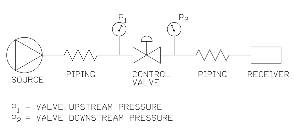
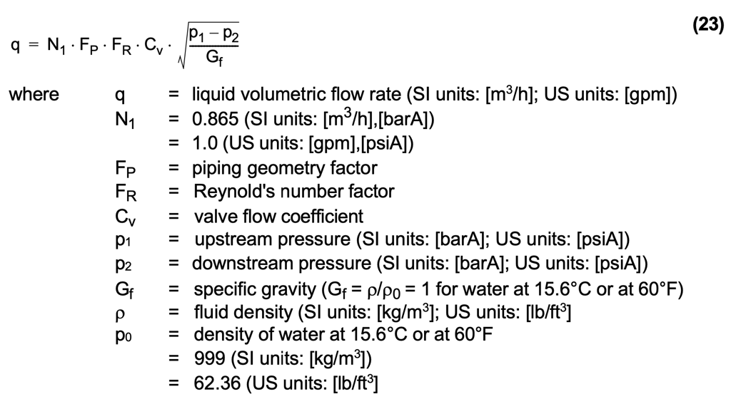
The following part of this manual concentrates on the throttling process between upstream pressure p1 and downstream pressure p2, as shown in figure 33, where upstream pressure p1 is the pressure measured by a tap located two pipe diameters upstream of the upstream valve flange, and downstream pressure p2 is the pressure measured by a tap located six pipe diameters downstream of the valve downstream flange (per std. IEC 60534/ISA S75).
To display the general behavior of flow through a control valve itself, the valve is simplified to an orifice in a pipeline, as shown in figure 34. Naturally, continuity equation (3) and Bernoulli's equation (4) are also valid in this context.
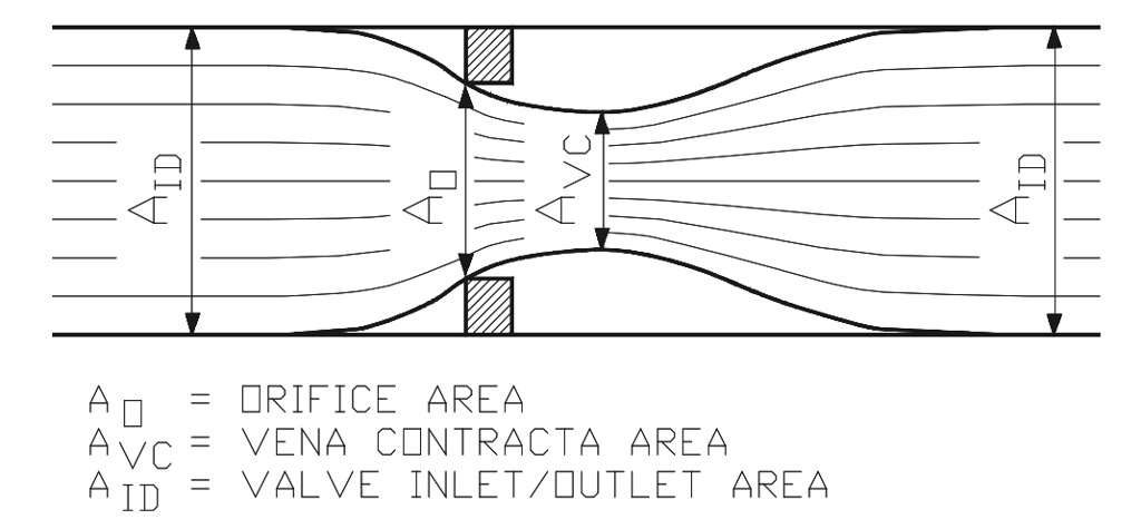
Figure 34. Flow through an orifice.
Figure 34 shows the change in the cross-section area of the actual flow when it goes through a control valve. In a control valve, the flow is forced through the control valve orifice, or a series of orifices, by the pressure difference across the valve. The actual flow area is smallest at the point called the vena contracta (AVC), the location of which is typically a little downstream the valve orifice, but can be extended even into the downstream piping, depending on pressure conditions across the valve, and on the valve type and size.
Due to the reduction in flow area, a significant increase in flow velocity has to occur to give equal amounts of flow through the valve inlet area (AID) and vena contracta area (AVC). The energy for this velocity change is taken from the valve inlet pressure, which gives a typical pressure profile inside the valve (figure 35).
The pressure inside the valve drops as the effective flow area is reduced, up to the vena contracta point, which is the smallest flow area available to the flow inside the valve. After reaching the vena contracta point the velocity of the flow is reduced due to the fact that more flow area becomes available to the flow. Thus some of the pressure lost up to the vena contracta point is recovered.
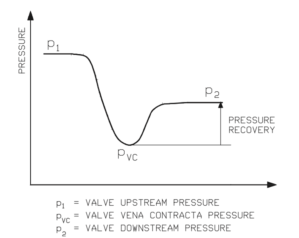
Figure 35. Pressure profile inside the valve in the valve trim.
The pressure recovery after the vena contracta point depends on the valve style and is represented by valve pressure recovery factor (FL), as given in equation (22). The closer the valve pressure recovery factor (FL) is to 1.0, the less the pressure recovery is.

When upstream pressure (p1) is constant, the interrelation between the pressure differential (∆p) across the control valve at a constant opening and the resulting flow rate (q) can be expressed by figure 36.
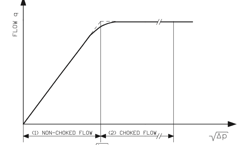
Figure 36. Interrelation between flow rate and square root of pressure drop across a control valve.
Up to a certain pressure drop value, the flow through a control valve follows the square root of the pressure drop applied across the valve in a direct line equation, where the slope of the line is expressed as the valve flow coefficient (Cv).
With larger relative pressure drops across the valve, the gain in flow decreases, and ultimately becomes zero. The cavitation begins where the flow starts to deviate from the straight line, as illustrated in figure 36. In other words, when upstream pressure (p1) is constant, an increase in pressure drop does not produce any increase in the flow rate through the valve. The cause of this phenomenon is choking. When the valve vena contracta pressure drops below the vapor pressure of the flowing liquid (figure 37), it causes formation of vapor bubbles in the control valve orifice, thereby restricting the liquid flow through the orifice.
The flow is considered to be choked when the valve's actual pressure drop is above the terminal pressure drop (∆pT), sometimes called the allowed pressure drop, derived as the corner point of the lines expressing non-choked and choked flows in figure 36.
In choked flow cases, where valve downstream pressure recovers above the liquid vapor pressure, a phenomenon called cavitation occurs. If the valve downstream pressure remains below the liquid vapor pressure, the phenomenon is called flashing.
3.2 Sizing equations for liquid flow
Liquid flow in non-cavitating or non-flashing conditions is given by equation (23).
With an increasing pressure drop (p1-p2), the vena contracta pressure in the valve drops below the vapor pressure of the liquid, and the vapor cavities begin to form in the liquid. At a certain point, when sufficient vapor has formed, the flow becomes completely choked, and the flow rate does not increase with increasing pressure drop, if upstream pressure is constant. The corresponding pressure drop is called the terminal pressure drop (∆pT).
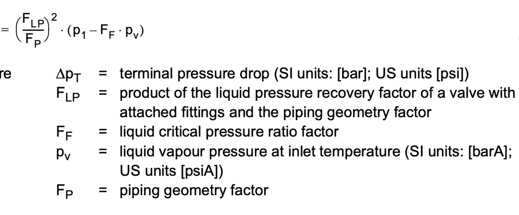
Consequently, the maximum flow rate (qmax) under choked conditions, is reached when (p1-p2) ≥ ∆pT
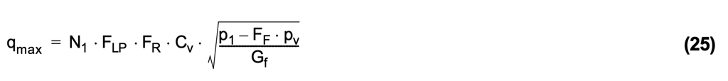
When a valve is operated in a way that the pressure drop is close to the terminal pressure drop (∆pT), the rate of flow may be less than that predicted by equations (23) or (25) because the real behavior of the flow rate is approximated using straight lines, as shown in figure 36. However, the error is insignificant.
Factors FF, FR, FP, and FLP
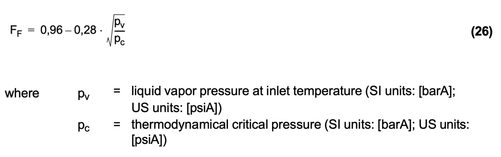
Factor FF, which is the critical pressure ratio factor for liquids, has an approximate value as given in equation (26).
Factor FR, which is the Reynolds number factor, usually has a value of 1.0. The Reynolds number factor has an effect in non-turbulent flow, which usually occurs with high viscosity fluids, such as oil, and with low flow velocities and small valve sizes. Reynolds number factor (FR) can be defined using the valve Reynolds number and figure 38. The valve Reynolds number is derived from the following equation (27).
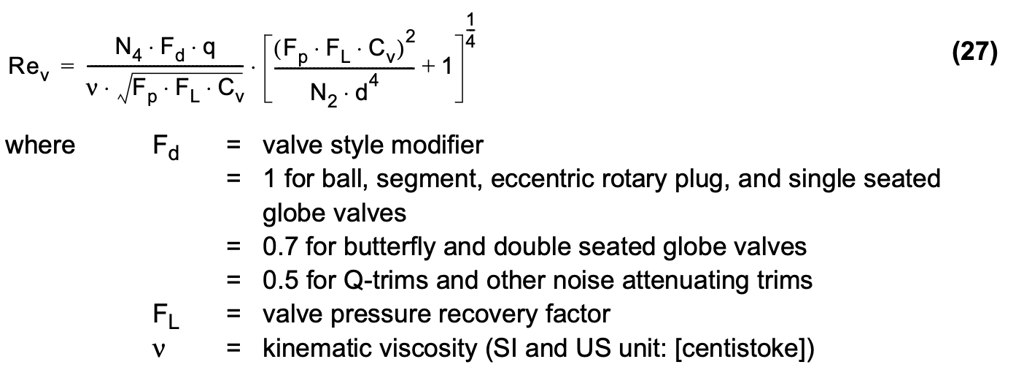
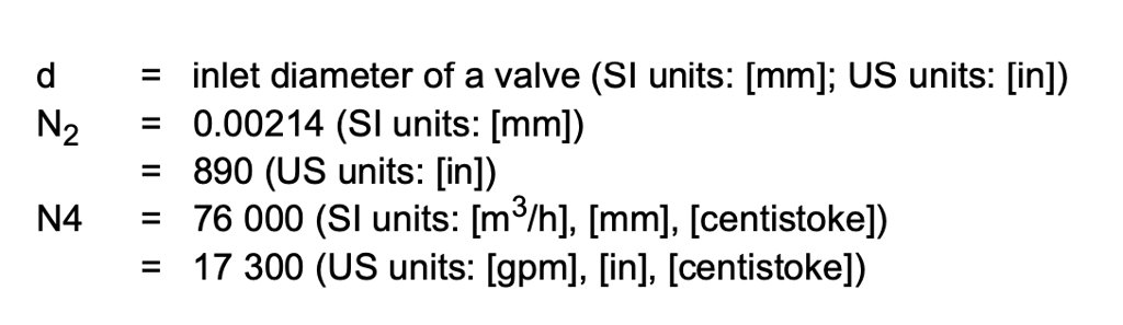
After calculating the Reynolds number for the valve (Rev), the Reynold's number factor (FR) can be determined from the diagram in figure 38.
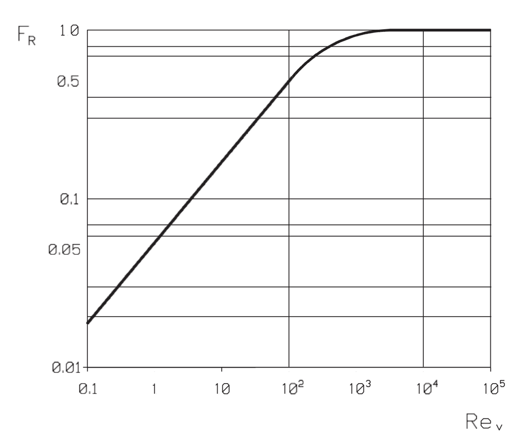
Figure 38. Reynolds number factor (FR) for liquid flow.
The piping geometry factor (Fp) can be calculated as shown in equation (28).
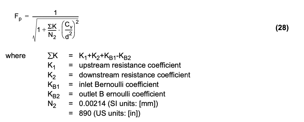
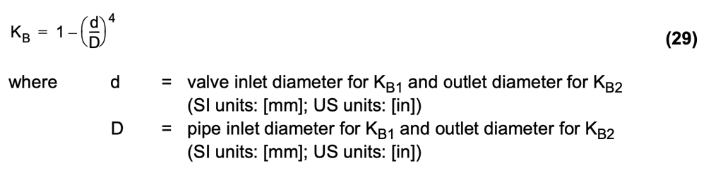
When the inlet and outlet fittings are identical, KB1 = KB2, they are canceled out in the equation. If the pipe diameters approaching and leaving the control valve are different from each other, the KB coefficients are calculated as in equation (29).
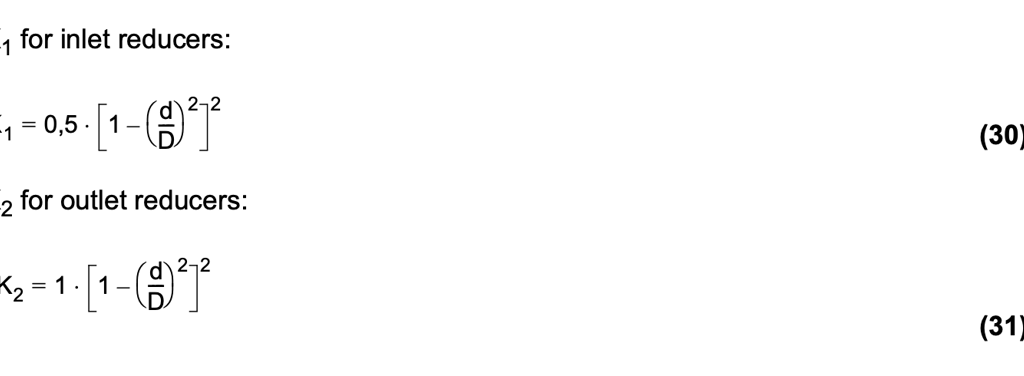
For standard concentric reducers, the upstream and downstream resistance coefficients (K1) and (K2) can be approximated as shown in equations (30) and (31).
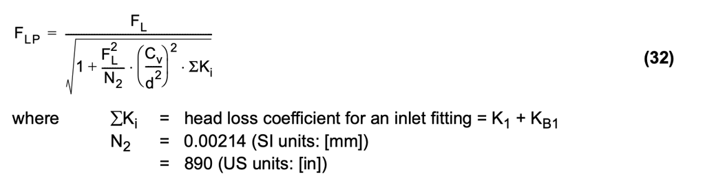
Factor FLP is the product of the liquid pressure recovery factor of a valve with attached fittings and the piping geometry factor (FP). It is calculated using the given valve pressure recovery factor (FL) and piping geometry factor (FP) as shown in equation (32).
3.3 Cavitation and flashing
3.3.1 Cavitation phenomenon
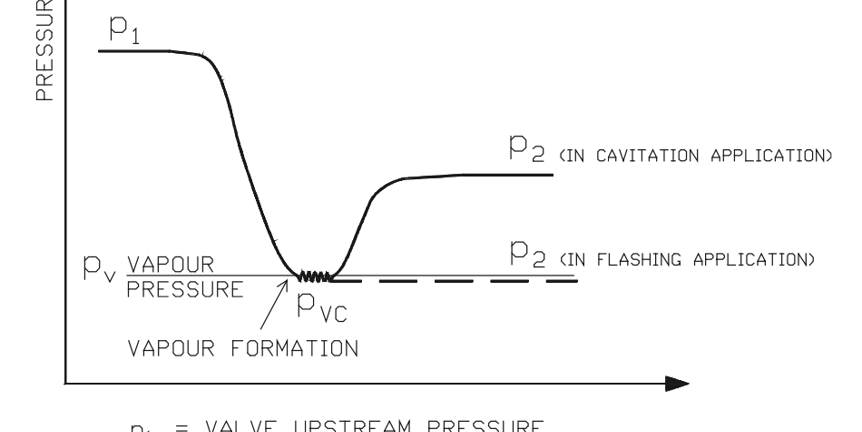
Cavitation is a two-phase phenomenon appearing in liquids under certain flow conditions. The cavitation within a control valve can most easily be described using figure 39, where changes in pressure and velocity conditions across a control valve are displayed using a simplified model of an orifice plate in the pipe.
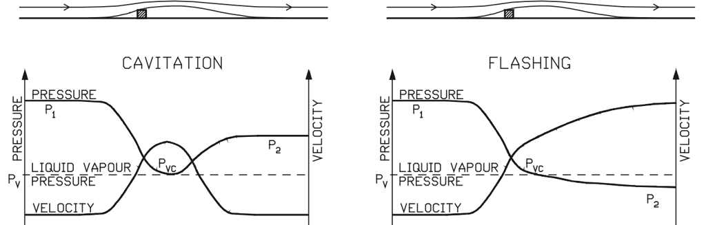
Figure 39. A simplified model of pressure and velocity changes in control valves in cavitating and flashing conditions.
A reduction in the area available for the flow leads to a large increase in fluid velocity, which in turn causes a drop in the fluid pressure due to the conservation of energy. The pressure is at its lowest level at the vena contracta point, which is located a little downstream of the physical valve orifice. When the pressure at the valve vena contracta point is lower than the liquid vapor pressure (pv) and the downstream pressure of thevalve (p2) is higher than the liquid vapor pressure (pv), cavitation takes place.
Cavitation occurs in two stages. During the first, the pressure of the liquid is reduced below the liquid vapor pressure, causing vapor bubbles to form in the liquid. The formation of vapor bubbles starts from boundary layers of the nuclei, minuscule solid particles, or gas bubbles that are carried by the fluid. In the second stage, recovery of pressure after the vena contracta raises the pressure above the liquid vapor pressure, causing a collapse of the vapor bubbles. As shown in figure 40 below, the collapsing vapor bubbles cause large pressure shocks, due to either a liquid microjet or a spherical shock wave.
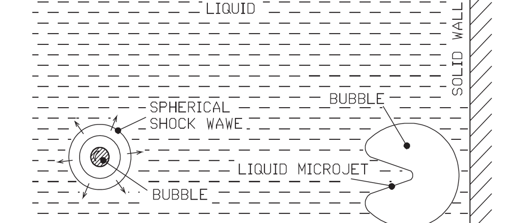
Figure 40. Pressure shock generation mechanisms.
If the vapor bubble is very close to or in contact with a solid wall, the generated microjet can hit the wall with a pressure shock of the order of 104 MPa (1.5 * 106 psi).
Spherical pressure shock waves are generated when bubbles collapse further away from solid walls and in the body of the liquid. In this case, the pressure shock is of the order 103 MPa (1.5 * 105 psi) and the effect of the microjet does not reach a solid wall. If bubbles collapse close to a solid wall, the microjet or shock wave can cause yield or surface cracks in the material. Cavitation-damaged surfaces are rough and spongy.
Figure 39 below shows a situation in which the valve outlet pressure is lower than the liquid vapor pressure. In a case like this, vapor bubbles cannot collapse and the fluid exits the valve as a two-phase mixture. The fluid is not cavitating, as the second phase (collapse of the bubbles) does not occur. This phenomenon is called flashing, and it is not nearly as damaging as cavitation. Selecting stainless steel valve body and trim materials, and limiting the flow velocity at the valve inlet and outlet typically gives satisfactory control valve life.
Mechanical damages to cavitating valves have been shown to closely correlate with the noise level produced. The maximum noise level is usually reached before the valve chokes. When choking and any flashing take place, the bubble collapse location and, thus, the source of noise, move further downstream. Cavitation damage also correlates with the materials and coatings used in the valve and downstream piping.
Although cavitation damage can be a purely mechanical phenomenon, it is often related to corrosion or erosion. In cavitation corrosion, the microjets or shock waves break the passivating film which is covering a metal surface. The existence of this passivating film is essential to the corrosion resistance of the material. The base metal is consumed in renewing this passivating film, and, as an ongoing process, this causes considerable loss of material from the cavitating location, as illustrated in figure 41.
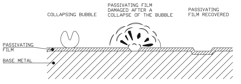
Figure 41. Wear on passivating film in cavitation corrosion.
Erosion related to cavitation or cavitation corrosion causes a substantial increase in material wear and damage. The metal material is softened by the joint effect of cavitation and possible corrosion, and thus is subject to wear by erosion. The erosion is strongly dependent on the flow velocity. Equation (33) expresses the relation between wear and flow velocity.
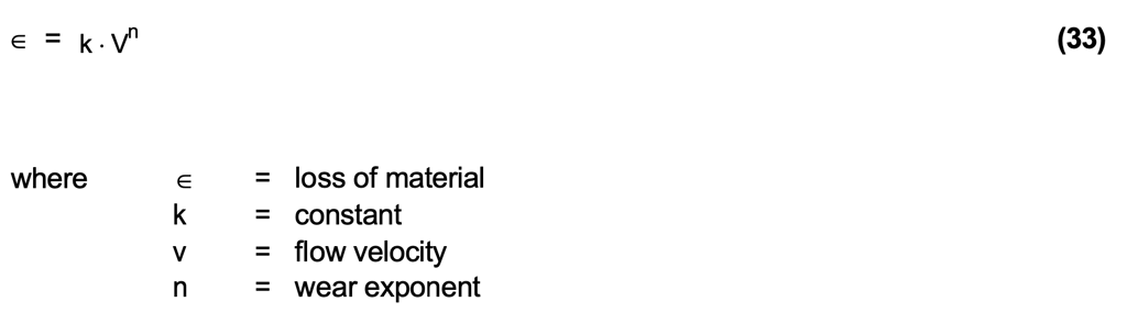
The value of exponent n in equation (33) can be as high as 7 in cases of erosion related to cavitation corrosion. In normal erosion, the value of exponent (n) is roughly 2.5. The wear is also strongly correlated with the materials used, with stainless steels suffering much lower wear than carbon steels.
In applications where cavitation exists, close attention should thus be paid to selecting the correct trim style and materials to avoid erosion related to cavitation corrosion. Equation (33) suggests the following:
- Reduce the flow velocity inside the valve by using multi-stage pressure drop trim to minimize valve trim velocities.
- Reduce the wear by using stainless and hardened materials.
3.3.2 Investigating the existence of cavitation
One way to estimate the level of cavitation is to use the pressure recovery factor (FL). The FL factor is determined according to the Cv measurement. The definition for the FL factor is shown in equation (22). On the basis of that equation, it is possible to calculate the terminal pressure drop for the valve. When the terminal pressure drop is reached, the flow is fully choked.
Some manufacturers publish a “cavitation index” (KC) for their valves. This number is the ratio (p1-p2) / (p1-pV). The value for the cavitation index is based on the Cv measurement with water. The point where the valve is considered to cavitate is the point where the curve in Figure 36 diverges 2% from a straight line. The value of the cavitation index varies with valve opening. The deviation is caused by cavitation, i.e. the valve is cavitating to some extent even before the limit set by the cavitation index is reached.
The intensity of the cavitation depends on the valve type and pressure level, so it is not easy to give an absolute limit for non-cavitating flow. For this reason, Valmet has decided to use both noise level and terminal pressure drop to predict cavitation level.
Cavitation and noise
Determining whether cavitation causes mechanical damage for a given set of flow conditions is complicated. Several different factors affect the degree of the cavitation damage: the valve material, the nature of the medium, pipeline layout, and possible solids in the flow. When the actual valve pressure drop is at or above the calculated terminal pressure drop, and the downstream pressure is higher than the vapor pressure, it is likely that significant cavitation damage will take place and any available means of preventing this should be used.
On the other hand, Figure 42 shows that cavitation starts before the terminal pressure drop is reached. The curve shows how the sound pressure level (SPL) of a valve develops as a function of the ratio (p1-p2) / (p1-pV). It can be seen from the next picture that the region of laminar flow is practically negligible, and noise levels are low. Following the laminar region, the curve is characterized by turbulence of the liquid flow and a moderate increase in the sound pressure level. From a certain value of the valve pressure differential, ∆p = z(p1-pV) onwards, the noise level curve starts to rise rapidly. The valve-specific characteristic pressure drop ratio (z) for incipient cavitation is determined by the manufacturer's laboratory measurement of hydrodynamic noise. These values are typically shown in the valve manufacturer's sizing coefficient documents. The reason for this increase in sound pressure level is cavitation. It can be seen from laboratory tests that the sound pressure levels start to rise even before actual steam bubbles can be visually observed.
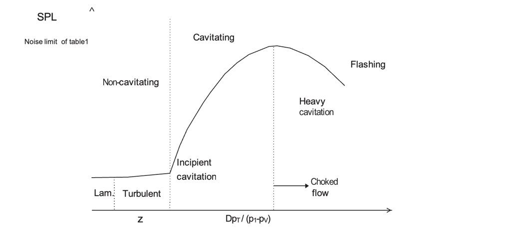
Figure 42. Liquid flow valve noise emission.
When the ∆p across the valve is close to the terminal pressure drop (∆pT), the sound pressure level reaches its maximum. Further increase in pressure ratio (p1-p2)/(p1-pV) will, as a rule, cause the noise pressure level curve to level off again, as can be seen from figure 42. This is predicted by the standard VDMA 24422 (1979) which, like most other standards, predicts the noise level one meter downstream from the valve. When the valve is heavily cavitating, the implosion of the cavitation bubbles occurs further away from the valve in the downstream piping. This is the reason for the reduction in sound pressure levels predicted by VDMA 24422 (1979). The noise does not disappear, but simply moves to another place (downstream piping).
Also, the length of the area where the implosions occur increases, so the intensity of the noise declines even though the number of bubbles increases. On the other hand, the nature of the flow more closelyapproaches that of a gas/liquid mixture when the pressure differential increases.
Typically, a valve which is noisy in liquid service is cavitating. Cavitation bubble implosions are the main source of disturbing noise, and noise level is directly related to cavitation intensity. In the early stages of cavitation (incipient cavitation,) the noise can sound like sand going through the valve. When the pressure difference across the valve is increased, the intensity of the cavitation rises and severe cavitation and rough noise occurs. Cavitation noise can also be accurately predicted. Therefore, the predicted noise level is a good indicator of mechanical cavitation damage.
The pressure drop needed to mechanically damage valves or piping depends on the type, size, and material of the valve. Various studies suggest that the lower the recovery of the valve, the closer the terminal pressure drop (∆pT) can be approached without cavitation damage. Terminal pressure drop (∆pT) occurs at a much higher level with a low recovery valve. It is not always true that when ∆p>∆pT, there will be damage. If the pressure differential is very small and the time that the valve is exposed to the cavitation is short, there may not be a problem. Corrosion is also a factor which depends on the material and the medium used.
There are two factors to consider when cavitation intensity is estimated:
- the pressure drop across the valve may not exceed the terminal pressure drop (∆pT) (If ∆p is small, ∆pT may be exceeded, but then the material selection is critical)
- the noise level of the valve may not exceed the values given in Table 1
Noise limits for preventing cavitation damage in valves for non-insulated schedule 40 piping are given in Table 1. It is important to note that even if the sound pressure level is below the limits given in Table 1, the valve might be cavitating heavily if the pressure difference over the valve is greater than the terminal pressure drop.
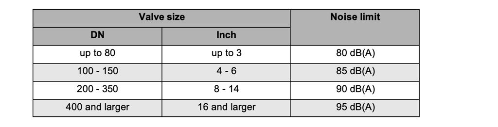
Table 1. Noise limits for liquid flow.
3.3.3 Flashing of liquids
When the downstream pressure of a control valve is less than the liquid vapor pressure, part of the liquid is vaporized and remains as vapor downstream of the valve. The flow downstream of the valve is part liquid and part vapor. The flow is choked, which is why a decrease in downstream pressure does not increase the flow rate. Flashing flow sizing is done according to liquid choked flow equations. In some cases where upstream pressure is very close to vapor pressure, flow may occur in two phases upstream of the valve, in which case the sizing is not as accurate. Two-phase flow sizing can be used in such cases.
Flashing flow may cause mechanical difficulties, like erosion and vibration. Unlike cavitation, the reason is the high velocity of the two-phase flow stream. High velocity is due to the larger vapor volume compared with liquid. High velocity can be very erosive and it is recommended that more resistant materials be used in such cases. Valve downstream velocity can be approximated according to the following calculations.
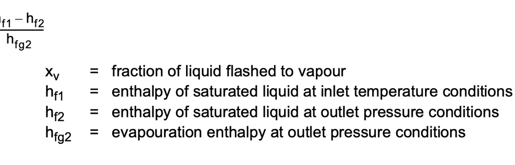
The amount of vapor in the flow stream is expressed as a fraction of flash, so that one hundred percent of flash is totally vaporized. The fraction of flash (xv) can be calculated from the enthalpy changes in the vaporizing process, as given in equation (34).
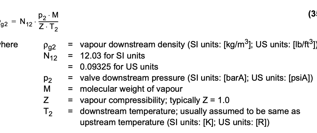
The density of the vapor in downstream conditions (ρg2), equation (35), is needed to calculate downstream velocity. Vapor density given for upstream conditions may be significantly different from the density in downstream conditions because of vapor compressibility.
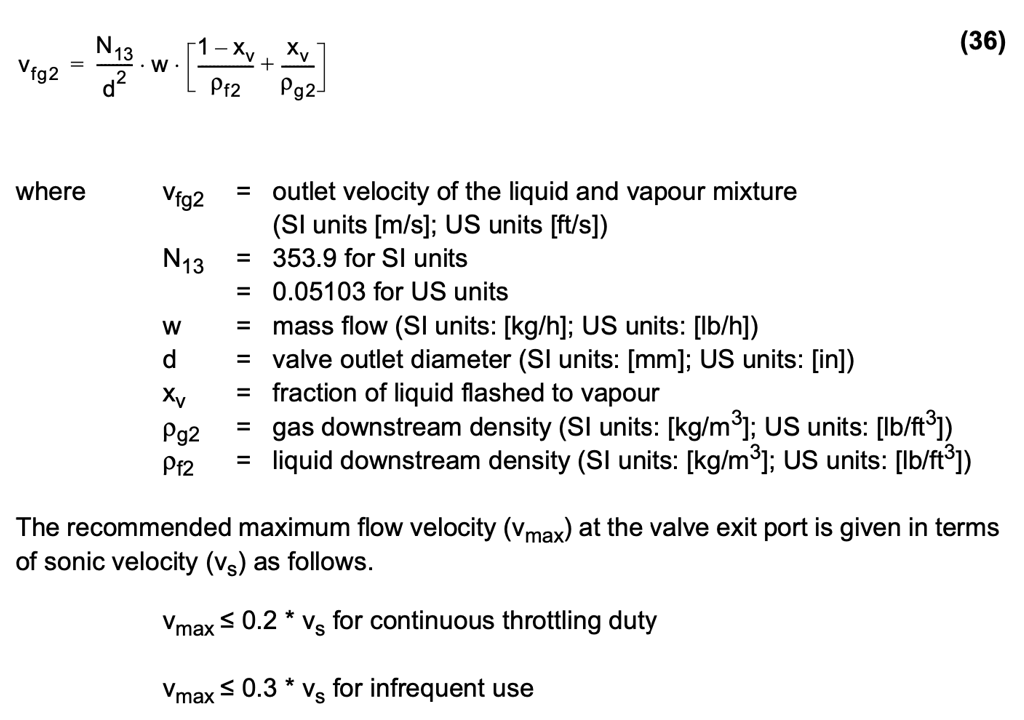
The outlet velocity of the liquid and vapor mixture (vfg2) can be calculated from equation (36).
In practice, it is recommended that the valve downstream piping length is minimized in flashing flow applications by locating the valve as close to the receiving vessel as possible. Vertical upward flow should be avoided to prevent any slug flow, which may cause strong vibrations.
There is currently no noise prediction method for flashing control valves. However, the noise level of control valves in flashing conditions generally stays below 85 db(A).
3.4 Cavitation and hydrodynamic noise abatement
The most significant source of control valve noise in liquid applications is cavitation. The abatement of noise and cavitation are therefore dealt with together in this section. In liquid valves, the basic division between methods of noise and cavitation abatement is between 'source' treatment, i.e. modification of the valve, and its trim, so that the cavitation intensity is reduced or the existence of cavitation is prevented, and 'path' treatment, i.e. dampening of the noise, generated. The source treatment of hydrodynamic noise and cavitation abatement can be performed using at least four different methods, as indicated in figure 43.
Source treatment, whenever possible and feasible, is the preferred way of dampening liquid cavitation and the associated hydrodynamic noise, because only then can excessive generation of cavitation bubbles be avoided across a wide flow range. Path treatment reduces the noise radiated by the piping system, but it does not eliminate cavitation inside the valve and adjacent piping.
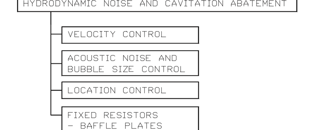
Figure 43. Hydrodynamic noise and cavitation abatement source treatment.
Velocity control
Controlling the fluid velocity, which is equivalent to controlling the pressure in the valve trim, is an effective means to avoid cavitation. For each liquid in question, the aim of this is to get the lowest pressure in the valve trim above the vapor pressure. This is done by dividing the valve pressure drop into several stages. There are two basic methods for pressure drop staging:
- identical pressure drop across each stage
- identical minimum pressure in each stage.
The first principle requires a constant flow area trim. Due to the equal area, the flow velocity at each stage is constant, and the pressure drop is equal in each step. The second principle involves an expanding-area trim, in which the pressure drop in the first stages is very high, but a higher minimum pressure is maintained in the last stages, thereby better avoiding cavitation within the valve trim. Figure 44 shows the two principles.
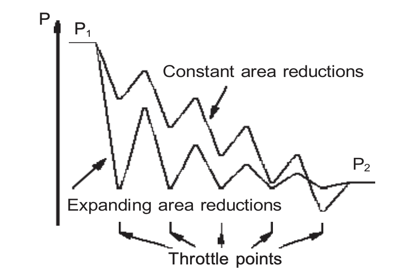
Figure 44. Alternative pressure staging principles.
An expanding-area trim is recommended when cavitation is to be eliminated to a very great extent. However, the velocity during the first stages of this trim will be quite high and may create erosion problems. In practice, valve designers usually combine the two methods to arrive at an optimum solution.
Acoustic noise and bubble size control
The division of flow into multiple small streams actually has two effects. Firstly, it acts to create a pressure stage. Secondly, it reduces the size of vapor bubbles in the fluid. Smaller bubbles cause higher frequency noise fields in the fluid and reduce the external vibration intensity of the pipe, as well as reducing the mechanical and erosion effects of cavitation. The concept of using small jets to reduce control valve noise is based on the principle that the jet produces a characteristic frequency above the pipe ring frequency, thereby reducing the sound reradiated by the pipe.
Location control
Location control is a principle of flow path design to overcomethe fact that that bubble implosions can be directed far away from solid boundaries.
Flat baffle plates
When the pressure drop ratio xF = ∆p/(p1-pV) becomes very high, it is possible that even a valve with an anti-cavitation trim cannot alone do a good job of reducing liquid cavitation and noise.
If the valve outlet pressure is increased with a baffle plate, the pressure drop ratio across the control valve can be brought back to the most effective valve operating range. The baffle plate is thereby used to create the required back-pressure for the valve.
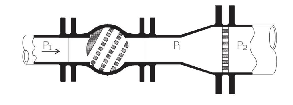
Figure 45. Typical installation of a noise attenuating valve with a flat baffle plate.
A flat baffle is a flow restrictor with a custom-made constant flow area and multiple holes for a particular flow condition. The pressure drop across a baffle plate is proportional to the flow squared. If it is assumed that the inlet pressure (p1) falls and the outlet pressure (p2) increases in proportion to the flow squared (cf. installed flow characteristics), the division of the total pressure drop (p1-p2) between the valve and baffle plate is described in figure 46.
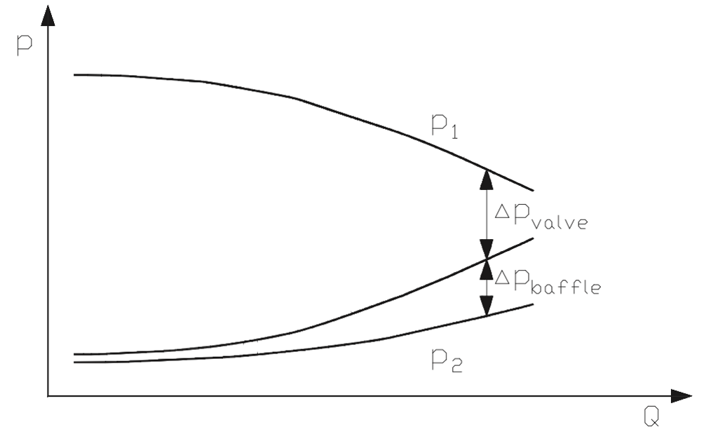
Figure 46. Typical pressure drop division between valve and baffle plate.
It has to be remembered that a baffle plate is a fixed restrictor, producing the desired pressure drop only at one given flow, namely that used for sizing the baffle. The baffle plates are typically sized for the valve maximum flow. As the flow is reduced, the pressure drop across the baffle decreases and the pressure drop across the valve increases. Thus, the baffle plate loses its effect at low flow rates.
Orifice plates
An orifice plate is a constant flow resistance. Unlike a baffle plate, there is only one large hole in an orifice plate, rather than multiple small holes.
An orifice plate can be used for producing linear valve installed flow characteristic, and, in limited cases, cavitation abatement. An orifice plate can be installed both upstream and downstream of a control valve. Sizing an orifice plate is basically similar to sizing a baffle plate.
Sizing baffle and orifice plates
The following instructions should be followed when sizing a baffle or an orifice plate downstream of the valve. The sizing is most easily done with sizing and selection software.
Choose a value for valve back pressure (pi) under maximum flow conditions. The capacity of the plate (Cv) can then be calculated using a pressure drop (pi-p2) as in equation (38).
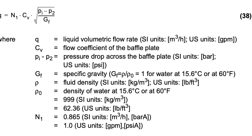
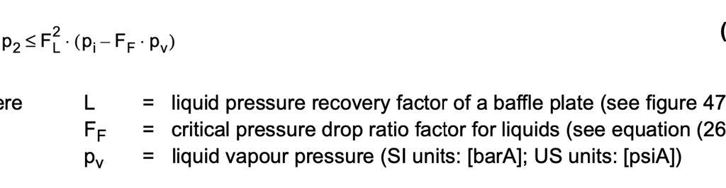
The chosen back pressure must ensure that the actual pressure drop across the plate does not exceed the terminal pressure drop of the plate, given by the equation (39). The calculation procedure may require iteration.
The pressure recovery factor FL of plates is shown in figure 47.
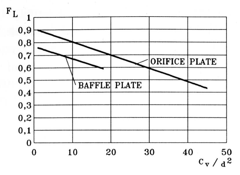
Figure 47. The pressure recovery factor FL for orifice and for baffle plates as a function of Cv /d2 (note that the nominal size (d) of the plate is in inches).
When the capacity of the plate is determined, the pressure drop across it at flows other than maximum flow can be calculated using liquid flow sizing equations. In non-choked flow conditions, liquid flow can be simplified as in equation (40).
For nonchoked flow, the required flow cross-section area for the plate can be calculated using equation (41).
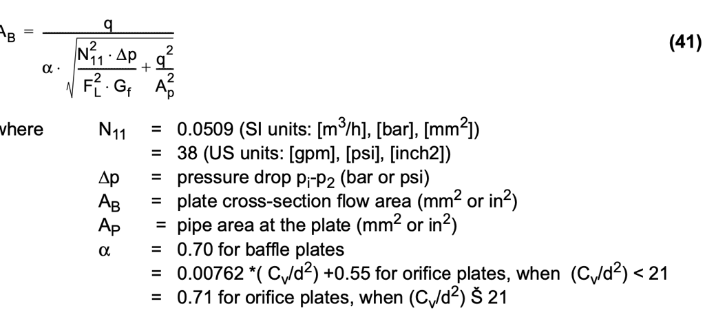
The maximum ratio of AB/AP for mechanical integrity of the baffle is approximately 0.4. Single orifices can have a larger area ratio.
In equation (42), it is shown how a single-hole orifice plate, when used upstream of the valve, is to be sized to ensure there is no cavitation.

The incipient cavitation coefficient (z) can be determined from figure 48. A higher cavitation coefficient (z) value for orifice plates compared to the value for baffle plates is due to a greater hole diameter ratio to the hole length.
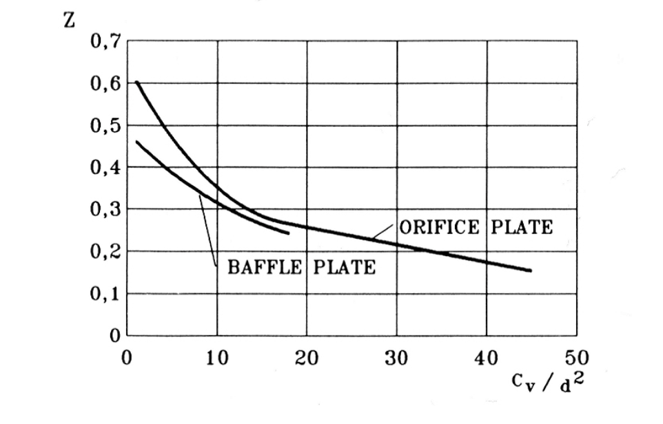
Figure 48. Incipient cavitation coefficient z for orifice and for baffle plates as a function of Cv/d2 (note that the nominal size (d) of the plate is in inches).
Example of noise and cavitation abatement
A Q-trimTM valve (figure 44) utilizes a combination of the effects described in the above paragraphs:
- The pressure drop is taken in multiple stages, leading to lower valve trim velocity and higher trim minimum pressure.
- Division of the flow into multiple streams diffuses the flow and provides acoustic control.
- The trim outlet is designed in a way that the flow is spread out evenly across the downstream flow port.
In rotary type of valves – like the one illustrated in figure 44 – the rotary motion gives additional benefits, such as being able to handle a very large flow range, and passing impurities through the valve.
3.5 Hydrodynamic noise prediction for valves
Noise generated by liquid flow is called hydrodynamic noise. At low pressure ratios, xF = ∆p/(p1-pV), with laminar or turbulent flow, the noise level is normally low. At a certain pressure ratio (xF=z), the noise level increases sharply. The reason for this sharp increase is cavitation. The value of cavitation coefficient (z) depends on the valve type and opening angle.
There are two well-known noise prediction methods used in the valve market. One is based on the German VDMA 24422 recommended practice which goes back to 1979 (see appendix K). The second method is an international standard for hydrodynamic noise prediction generated by a control valve, IEC 60534-8-4.
According to the VDMA 24422 (1979), the noise level in dB(A) can be calculated using the following equations (equation (43) for SI units and equation (44) for US units) when the flow is turbulent but cavitation has no effect on the noise level; (xT < z). In equations (43) and (44) ∆LF = 0


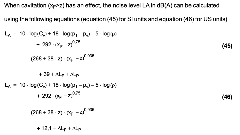
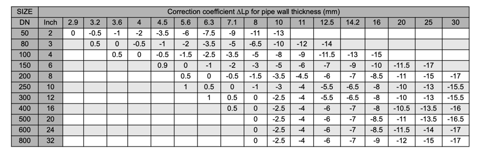
For each valve, the z and ΔLF values for equations (45) and (46) are usually presented in the manufacturer's Cv tables and noise prediction graphs. Correction coefficient ∆LP is the correction for pipe attenuation and is given by the following graph (figure 49) and table 2.
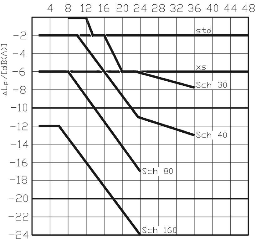
Figure 49. Correction coefficient ∆Lp for pipe schedule number.
As a general rule, hydrodynamic noise prediction according to the IEC 60534-8-4 is more laborious than that of the VDMA 24422 (1979). Noise prediction is based on a method where mechanical stream power as well as acoustical efficiency factors are calculated in different flow regimes, i.e. turbulent and cavitation conditions. The sound pressure level inside the pipe is estimated and the pipe external noise attained from the inner sound pressure level by reducing the transmission loss of the piping.
In short, IEC hydrodynamic noise prediction can be presented in the five following steps:
- The noise source is the mechanical energy dissipated in the valve. The mechanical stream power is calculated at the vena contracta of the valve.
- A small part of mechanical power is transferred to acoustical energy. The portion of the mechanical power converted to (acoustical) sound power is defined by using acoustical efficiency factors. Different flow regimes (turbulent and cavitation) have different acoustical efficiency factors.
- The sound power is converted to internal sound pressure level at the downstream of the valve. The peak frequency of the generated noise is also estimated.
- The transmission losses of the piping are defined. The transmission loss is dependent of the piping, the peak frequency and the fluid properties. Step 4 also covers the part where the pipe external sound power level is A-weighted.
- Define the A-weighted sound pressure level at the observation point at a distance of 1 m from the pipe wall.
3.6 Hydrodynamic noise prediction for baffle and orifice plates
The valve and baffle or orifice plate noises are first calculated separately using the VDMA 24422 noise prediction standard. The valve sizing and noise prediction is done using (p1-pi) as the pressure drop for the valve. Pressure pi is the intermediate pressure between the valve and the plate. The required capacity (Cv) for the baffle plate is calculated with the IEC 60534/ISA S75 sizing equations for liquids, using (pi-p2) as the pressure drop for the baffle. The pressure recovery coefficient (FL) and acoustical coefficient (z) are given as a function of Cv/d2. The hydrodynamic noise coefficients (∆Lf) for the orifice and baffle plates are given in figures 50 and 51.
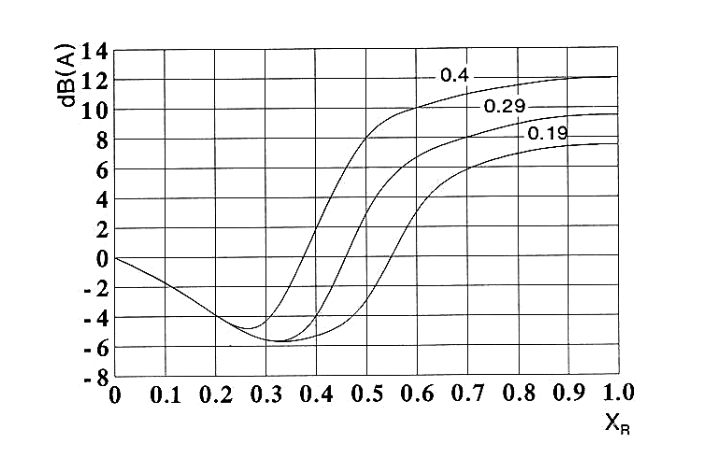
Figure 50. Hydrodynamic noise coefficient ∆Lf for baffle plates as a function of XR = (x-z) /(1-z), the three curves representing different ratios of baffle-free cross-section area to pipe cross-section area.
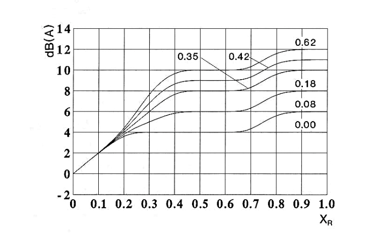
Figure 51. Hydrodynamic noise coefficient ∆Lf for orifice plates as a function of XR =(x-z)/(1-z), the six curves representing different ratios of orifice-free cross-section area to pipe cross-section area.
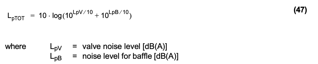
The total noise LpTOT is calculated by adding the noise levels from different sources logarithmically as in the following equation (47).
3.7 Recommended flow velocities for liquids
Limitation of liquid flow velocity in pipelines and control valves is mainly used to prevent excessive erosion. Other reasons include piping pressure losses (proportional to velocity squared), and corrosion (wearing away of protective film from metal surface). In the case of butterfly valves, high inlet velocities can also lead to instability of the valve trim.
The following are recommended inlet velocities for liquid service control valves:
- Segment, ball, globe, eccentric rotary plug, and Q-trimTM valves:
- Inlet velocity ≤ 10m/s (32 ft/s) for continuous duty
- Inlet velocity ≤ 12 m/s (39 ft/s) for infrequent duty
- Butterfly valves:
- Inlet velocity ≤ 7 m/s (23 ft/s) for continuous duty
- Inlet velocity ≤ 5 m/s (27 ft/s) for infrequent duty
Typical piping design velocities range from 2 to 3 m/s (6 to 10 ft/s) for liquids.
The above values are for relatively pure liquids. As well as cavitation and flashing, impurities in the flow may reduce the allowed maximum flow velocities.