2 Control Valve installed performance

2.1 General
In this chapter, we introduce a process pipeline model and calculation procedure enabling the quick and accurate prediction of control valve installed performance using a valve sizing and selection software. Choked flow conditions are taken into account for all calculated points, a factor that was listed as a limitation in previously presented models. The results and their utilization are discussed in detail, with practical guidelines on how to correct nonlinear installed flow characteristics using a digital controller signal modification block.
It is also important to note that control valve installed accuracy is the method that should be used to judge control valve accuracy, not just the mechanical accuracy. The installed gain multiplied by the mechanical accuracy gives the installed flow accuracy.
2.2 Operating conditions
Successful control valve sizing and selection depend on knowing the actual process conditions in the system in which the valve is to be installed. It is known that distinct information on operating conditions very seldom exists. The more assumptions one has to make on flow conditions, the less accurate the control valve sizing is going to be. Fortunately, when a few flow conditions are known accurately, an algorithm can be found that can model the behavior of a given control valve for the whole flow range.
2.3 Selecting a control valve
The selection of a control valve is divided into two parts. Firstly, there is the mechanical selection in which suitable valve style, materials, and pressure rating are picked to guarantee safe and reliable performance according to good engineering practices, local laws and regulations. This selection should be made using bulletins and technical information specific for each valve type. Secondly, there is the sizing of a selected valve, where the size of the given valve type is determined while trying to prevent unwanted phenomena like excessive noise or liquid cavitation. After the valve size has been determined, the installed performance of the valve to phase out poor control performance – like hunting, excessive slow or fast response and poor accuracy – is further predicted.
This control valve selection concentrates on sizing and installed performance considerations. It should be noted that these calculations do not, by themselves, guarantee the selection of a correct valve. Therefore, careful mechanical and material evaluations should always precede sizing calculations.
2.4 Control valve flow characteristics
In the past, selection of control valves has largely been based on approximate estimation methods and practical experience. Modern sizing and selection software enables faster and more accurate calculation methods to select a control valve with optimum controllability and accuracy for each individual process application. The method is based on modeling or predicting the actual flow characteristic and gain of the installed valve.
2.4.1 Inherent flow characteristic
Selection of the optimum size and type of a control valve starts with the valve's inherent flow characteristic. For this reason, all control valve types must be laboratory tested to determine their exact inherent flow characteristics.
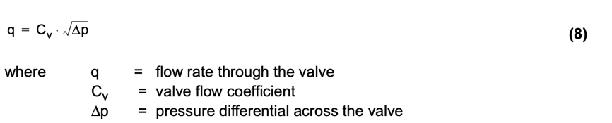
Valve inherent flow characteristics are defined to keep the pressure differential across the valve (∆p) constant. As the differential pressure (∆p) is constant, the flow rate (q) through the valve is proportional to the valve flow coefficient (Cv), as expressed in the simplified equation (8).
Because the valve flow coefficient (Cv) reflects the effective flow cross-section of the valve, the valve inherent flow characteristic shows how the effective flow cross-section changes as a function of relative travel (h).
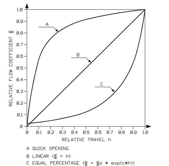
Figure 16 shows the most common valve inherent flow characteristics. The relative flow coefficient (F) is determined as shown in equation (9).
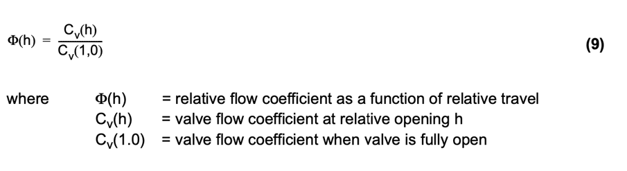
The inherent flow characteristic is the shape of a flow curve through the valve, with a constant pressure drop across the valve. Note that in any case where process piping is attached to the valve, the piping pressure loss, a function of flow rate, will cause the valve pressure drop to vary as a function of the flow rate, even if the pressures at the source and receiver are constant.
A. Quick opening inherent flow characteristic
A flow characteristic in which a flow close to a maximum is reached with a very small opening. Most commonly used in globe valves for on-off services and in cases where only a limited stroke is available due to the nature of actuator, as in the case of pump governors.
B. Linear inherent flow characteristic
A flow characteristic in which the valve relative opening directly correlates with the percentage flow. For example, a 50% open valve gives 50% of maximum flow, with a constant pressure drop across the valve. If the pressure drop across the valve remains absolutely constant independent of the flow, this will be an optimal inherent flow characteristic, because in that case the inherent flow characteristic equals the installed flow characteristic.
C. Equal percentage inherent flow characteristic
A flow characteristic in which equal increments in the valve opening cause a constant percentage increase in flow with a constant pressure drop across the valve. It is designed to linearize the installed flow characteristic in normal control valve applications, where the amount of pressure drop available to the control valve decreases with the opening of the valve, due to the increase in pressure losses in other parts of the system, such as pipes, pumps, heat exchangers etc.
2.4.2 Installed flow characteristic
Under operating conditions, a control valve is part of a process pipeline. In the valve travel range, the differential pressure across a valve is seldom constant because dynamic pressure losses in the flow cause the valve inlet pressure to fall and the outlet pressure to rise as the flow rate increases. For an installed valve, the dependence of the flow rate (q) on the travel (h), i.e. the shape of the installed flow characteristic curve, is therefore a function of the process pipeline and of the inherent flow characteristic of the valve. The changes in differential pressure that take place across a control valve installed in a process pipeline are illustrated in figure 17.
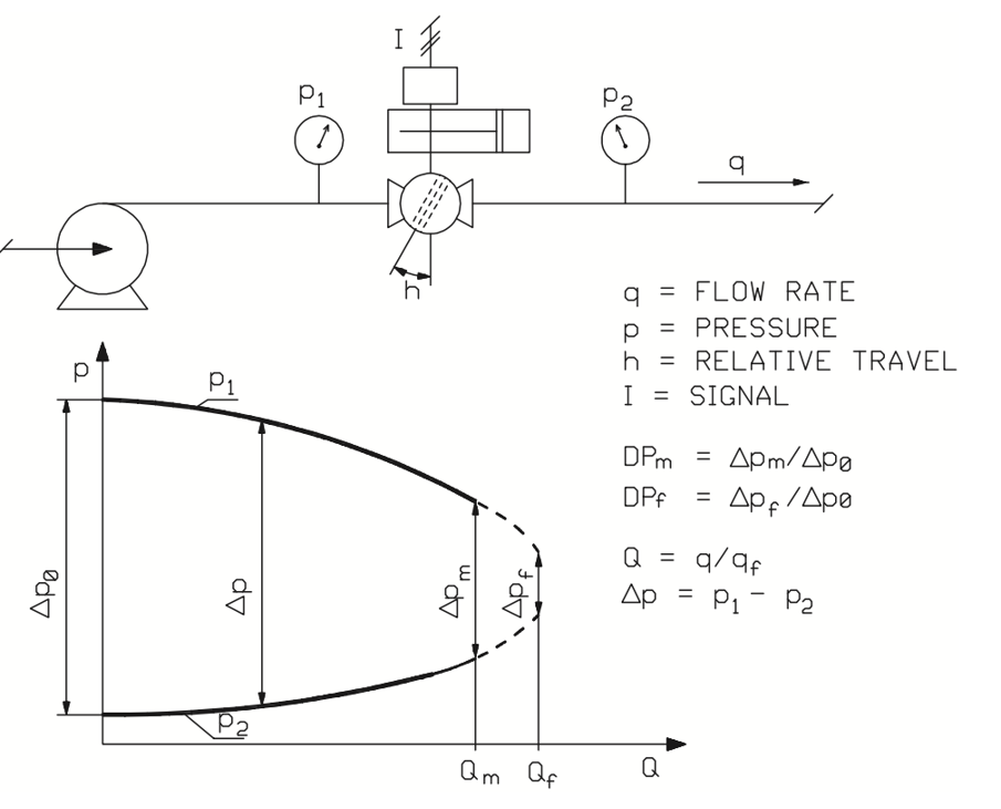
Figure 17. Change in effective differential pressure across the valve due to a change in the flow rate.
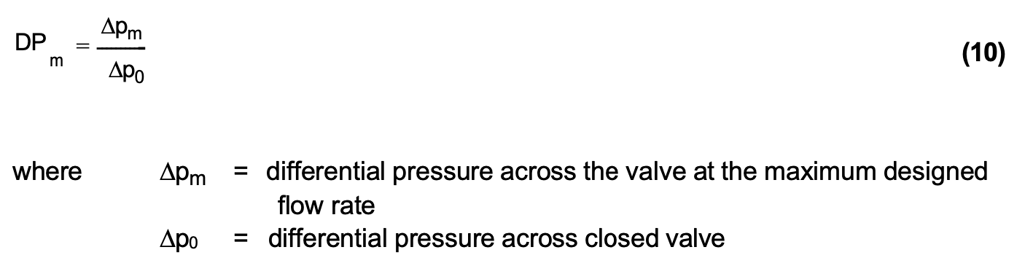
The character of a process pipeline is described by the process pressure ratio factors DPf or DPm. The subscripts refer to situations in which the valve is fully open (subscript f) or opened to enable the maximum flow rate (subscript m) required by the process. The process pressure ratio factor DPm is the differential pressure across the valve at the process maximum flow rate divided by the differential pressure across the valve when the valve is closed, as expressed in equation (10).
The character of the process pipeline can be determined with sizing and selection software when at least two different flow conditions in the process are known or if the process pressure ratio factor DPm describing the character of the pipeline and the maximum flow conditions are known.
The process pressure losses are relative to the square of the flow velocity, which corresponds to the square of the flow rate. This basic assumption facilitates the creation of a model for pressure variations at the valve inlet and outlet.
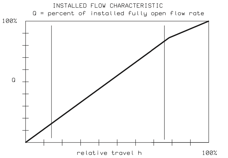
Figure 18 shows an installed flow characteristic curve, calculated using a sizing and selection software for an eccentric rotary plug control valve, in a process application.
2.4.3 Installed gain
The quality of the installed flow characteristic curve with respect to valve controllability and accuracy can be examined by the means of a valve gain curve. It describes the changes that take place in the slope of the installed flow characteristic curve for different amounts of valve travel. The gain of an installed valve is the change in relative flow rate (dQp = d(q/qm)) divided by the change in relative travel (dh), as expressed in equation (11).

The installed gain gives the rate of change in flow as a function of the change in signal. A gain of 1 means that a 1% change in the valve opening causes the flow to change by 1% of the maximum flow. A gain of 2 means that a 1% change in the signal causes a 2% change in the relative flow rate (dQp), and so forth.
The change in flow rate (dQp) can be expressed as in equation (12).

In other words, the change in flow rate (dQp) is the gain (G) multiplied by the change in valve travel (dh).
From equation (12), it can be seen that variation of the gain (G) in the required flow range causes different relative flow changes (dQp) for the same relative signal change. This is usually undesirable for process controllability.
The installed valve gain is the starting point for selecting an optimum control valve size and an inherent flow characteristic for a certain process application. For the standard PID controllers in most control loops the best possible inherent flow characteristic is the one that gives closest to constant installed gain for the required flow range. In this case, the controller's parameter tuning can be kept optimal and unchanged in spite of variations in the load in the process operating range. In applying the above rules, it must, however, be noted that only a full dynamic analysis of the control loop is sufficient to include all the nonlinearities of the process and equipment and to absolutely guarantee the choice of an optimum control valve. This kind of analysis is feasible for a control valve simulation program.
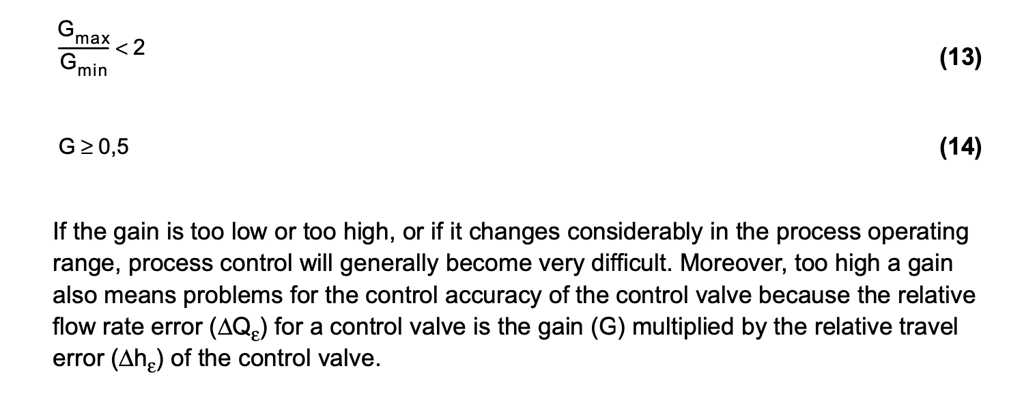
The rule of thumb for permissible limits for the installed gain is that a change in gain larger than 2 (equation (13)), or a relative gain smaller than 0.5 (equation (14)) should be avoided in the process operating range.
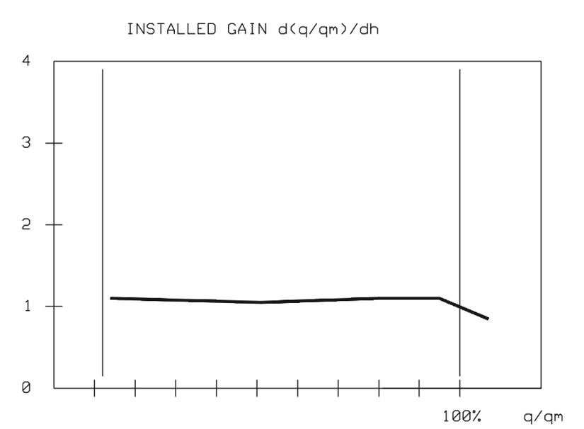
Figures 19 and 20 illustrate the importance of selecting the proper size control valve for each application. An oversized control valve causes high gain with small flows resulting in poor control accuracy and possible hunting, as shown in figure 19. Selecting a smaller valve will lower the gain, resulting in high accuracy and stable control, as shown in figure 20.
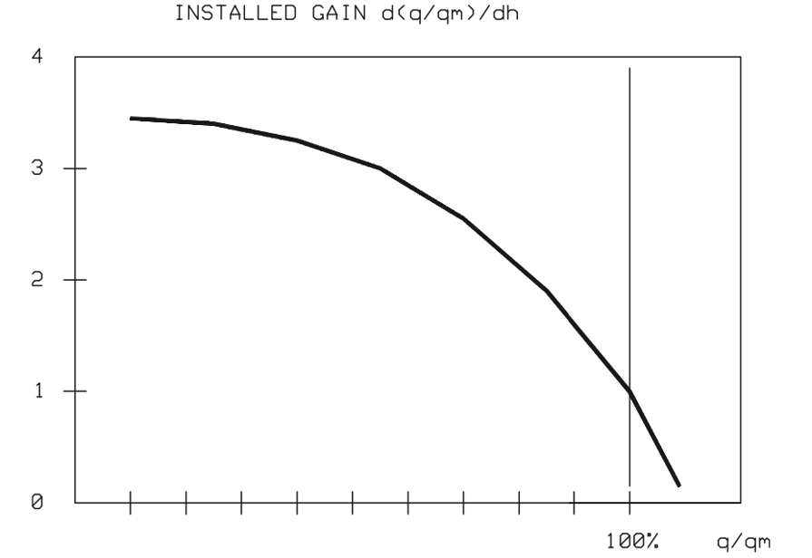
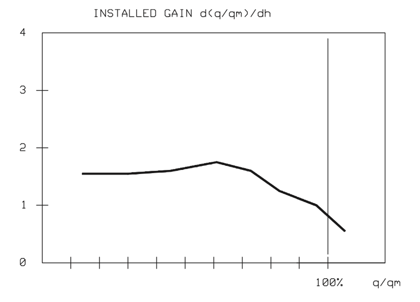
Figure 21 shows a sample installed gain curve for a new type of eccentric rotary plug control valve. The figure demonstrates that an almost constant gain is achieved on the inherent flow characteristics of the eccentric rotary plug control valve. This is often the optimum gain in the process operating range. Furthermore, a smooth gain results in excellent control accuracy.
2.4.4 Calculation methods
With sizing and selection software, it is possible to predict the installed control valve flow characteristic and gain curves if at least two separate sets of flow conditions or if the process maximum flow and DPm factor are known.
The program accurately predicts installed control valve performance if the following conditions are true:
Condition 1: The process is such that a specific flow corresponds to a specific pressure drop across the valve.
Condition 2: Pressure drop changes across the control valve are dependent on pressure losses in the piping system such that the sum of those pressure losses is proportional to the square of flow velocity.
The program uses following procedures to calculate the installed flow characteristic and gain:
- Using given flow data the program generates a process model for the pressures, and checks whether conditions 1 and 2 above are fulfilled. The process model for the valve inlet and outlet pressures is created using 'the sum of least squares' method such that the derivative equals zero at the origin of the pressure
- The program predicts the flow through a fully open control valve (qf) using the process model to determine pressure drop across the fully open control valve. Possible choked liquid flow, determined by pressure recovery factor (FL), or critical gas flow, determined by pressure drop ratio factor (xT), are taken into account when determining flow through a fully open control valve (qf).
- The valve pressure drop, opening and predicted noise level for the whole flow range are calculated at intervals of 5% of the maximum flow (qf). At each of the calculation points possible choked flow is taken into account in the The installed flow characteristic displayed on the screen is the relative flow rate (q/qf), which is the actual flow rate divided by the flow in a fully open valve, given as a function of relative travel (h).
- The installed control valve gain is the slope of the installed flow characteristic curve defined using finite difference method. It is important to note that the installed gain curve is calculated and drawn as a function of the maximum process flow (q/qm) and not as a function of the flow with the valve fully open (q/qf). This is important, as it allows different valve types and sizes to be compared based on process requirements, and not just from the valve It is worth mentioning, that this method increases the gain as compared with the gain presented as a function of flow in a fully open valve.
Process model and DPm selection
In order to calculate the installed control valve flow characteristic and gain, a model of the process according to which the pressures involved in the process piping change has to be available, since the program determines the process model based on flow data. In most cases the model of process pressures used is such that the pressure drop across the control valve decreases with increasing flow caused by opening the control valve.
The pressure behavior of the process can be estimated accurately enough for practical purposes, when the pressure conditions (upstream pressure, pressure drop across valve) and flow rates are known for at least two flow conditions, such as the maximum and minimum flows. If only the maximum flow for the process (qm) and the corresponding pressure drop (∆pm) are known, the process model can be found by using the process pressure ratio DPm, as in figure 22.
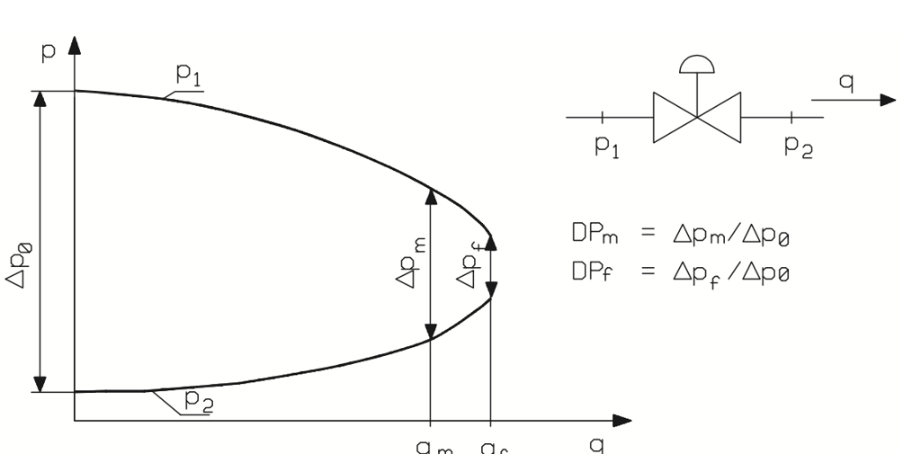
Figure 22. The process pressure model.
DPm is the valve pressure loss portion of the total dynamic pressure loss of the system with maximum process flow. The DPm information should thus be easily available from system pressure loss calculations.
The program is able to calculate the pressure process model using two or more given flow conditions if these flow conditions comply with conditions 1 and 2 of the procedure. Figure 23 gives examples of defined process models the program can handle, and that of undefined process models that it cannot.
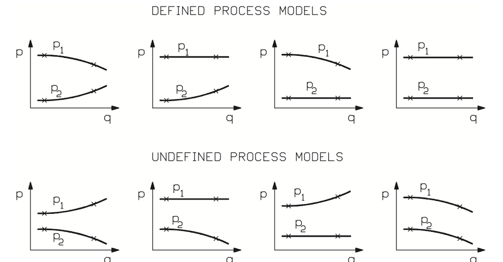
Figure 23. Examples of defined and undefined process models.
The process pressure ratio DPm is affected by the dynamic pressure loss in the piping. The piping pressure loss is generated by the length of the pipe, the diameter, surface roughness, and individual resistances of piping components. Additionally, the pressure drop across a control valve depends on the flow velocity and piping boundary conditions, e.g. if the fluid is a liquid, the pump curve needs to be taken into account when evaluating the change in pressure drop across the valve.
DPm ratio gives the program user a chance to evaluate and optimize piping structure options and the effect different valves have on overall process total function. The DPm ratio can be optimized such that a minimum amount of energy is used in the control valve, leading to significant saving in the energy cost of pumping. The following A and B give examples of the selection of DPm ratios for liquids and gases.
A. Liquid flow
In practice, most process piping systems are now designed such that the control valve pressure loss at maximum designed flow is roughly one third of the total dynamic pressure loss in the piping. In that case, DPm ratio as a rule of thumb for liquid piping is as presented in equation (15).

As mentioned before, piping designers are an invaluable asset in calculating the real DPm factor, particularly for new piping systems. Old systems can be evaluated using common sense to determine a DPm ratio accurate enough for present purposes. Figure 24 presents an estimation of DPm ratio in two different kinds of process piping.
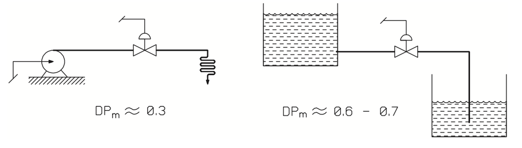
Figure 24. Evaluating DPm ratio for liquid flow.
B. Gas Flow
For compressible flows, such as those of gases and steam, the pressure drop changes across a control valve are usually smaller than those for liquid flows. The difficulties involved in presenting 'rules of thumb' for gas and steam flows are, firstly, that there is huge variation in different process and piping systems and, secondly, that fluid compressibility, particularly at large flow velocities, has a big effect on the pressure drop across a control valve. Equation (16) gives 'a rule of thumb', which can be used when no accurate information is available.

Trying out several possible DPm ratios to view the effect this has on the installed flow characteristic and gain is suggested in such cases. Some example estimates for DPm ratios for gas or steam flows in different process piping systems are given in figure 25.
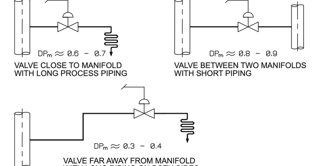
Figure 25. Evaluation of DPm ratio for gas and steam flows.
2.4.5 Control valve accuracy
A control valve in a control loop determines much of the quality of the overall control loop function. Specific attention should thus be paid to control valve selection in order to get the full benefits of the extensive product development that has occurred in other components of the control loop, such as measuring devices and DCS process control systems.
A control valve is the final control element, a mechanical device that effects the changes in flow or pressure deemed necessary by the rest of the system. Therefore, the control valve accuracy is a main element in defining the accuracy of the whole control loop.
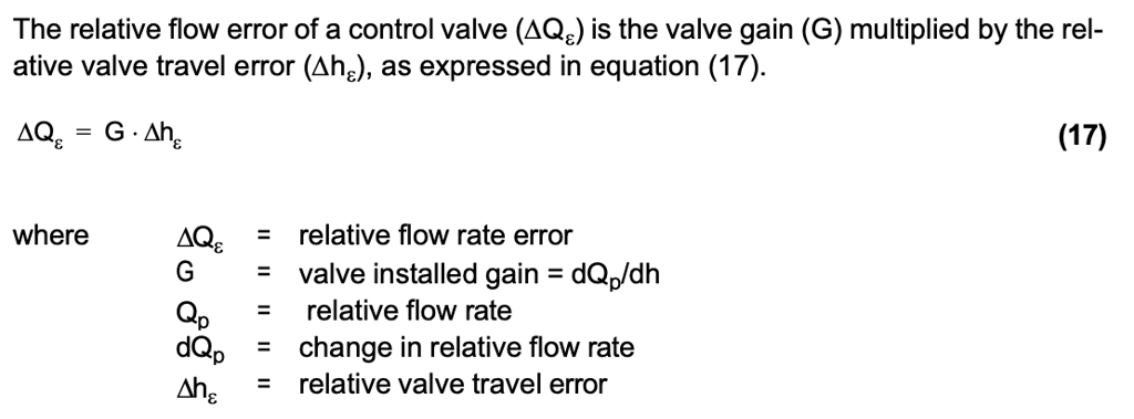
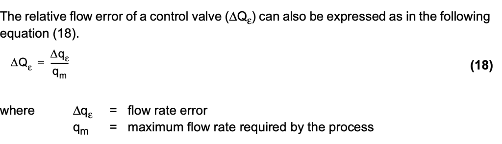
The installed gain (G) in the equation (17) is the control valve installed gain which can be calculated by sizing and selection software.
The accuracy of the flow controlled by a control valve is the mechanical error of the control valve assembly multiplied by the installed flow gain. A figure for the mechanical error alone does not indicate the accuracy of the flow being controlled.
2.4.6 Control valve characterization
The inherent flow characteristic of a control valve is traditionally chosen so that in the process operating range, the controller tuning can be kept constant in spite of load changes. If the process being controlled is nonlinear, the control valve flow characteristic should, inversely, be nonlinear. Thus the control valve flow characteristic will compensate for a nonlinear process.
The rapid development of process control systems has, however, made it possible to apply highly developed control strategies and algorithms. In this case, there is a tendency to select various subsections of the control loop to be as linear as possible in the process operating range. For control valves, this can be done by selecting a valve type and size that give a linear installed flow characteristic and constant gain in the given process flow range.
In certain applications, due to accuracy requirements or process conditions, the desired installed flow characteristics or gain cannot be achieved with the normal range of valves. In this case, the flow characteristic of the valve can be modified using characterization, as illustrated in figure 26.
Most control systems assume that the installed flow characteristic of the control valve is linear. Therefore, for optimal performance of the control valve, measures should be taken to ensure installed flow characteristic are as close to linear as possible by selecting the valve style and type accordingly.

Figure 26. Control valve characterization by modifying controller output.
Characterization of control valve performance can basically be achieved in four different ways, namely, by modifying:
- the controller output, as in figure 26
- the signal in the positioner
- the valve control orifice, the plug, or both
- the slope of the analog positioner feedback cam or use of the characterization feature of the digital positioner.
Figure 26 shows the control valve characterization performed by controller output modification in the case where a constant gain is required for the control valve. In this case, the control valve is fitted with an electropneumatic positioner with a linear feedback cam.
The controller characterization curve in figure 27 can be plotted using sizing software when the installed flow characteristic graph relative flow rate (Q) is replaced by the input signal (I) for the linearization block, and relative travel (h) is replaced by the output of the linearization block (Imod):
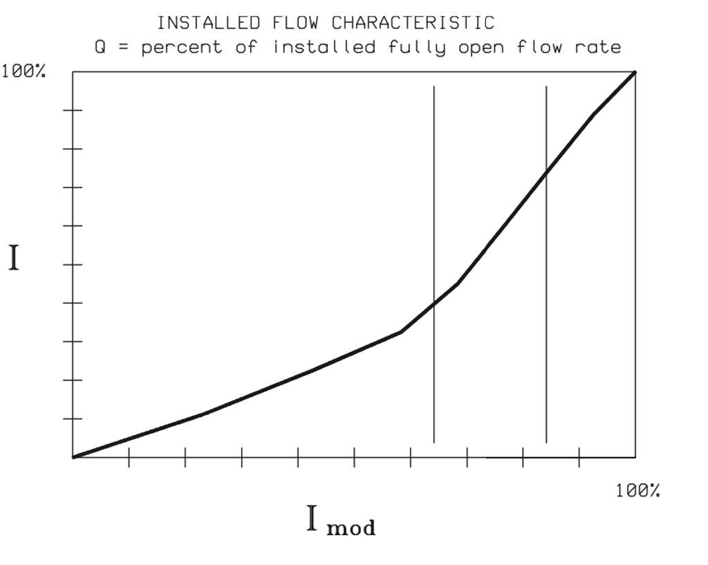
Figure 27. A characterization curve produced from a sizing software.
Modern process controllers are capable of linearizing the control valve installed characteristic by signal modification. This method, which is applied by using a graph like the one shown in figure 27, provides accurate linearization for the particular application.
Positioner cam modification simply distorts the valve inherent flow characteristic without taking into account the actual requirements of the specific system considered.
Modification of control valve characteristics by modifying the positioner feedback cam can be studied using the block diagram in figure 28.
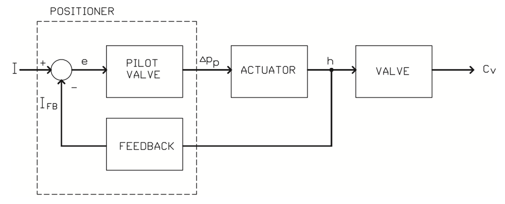
Figure 28. Block diagram for a control valve.
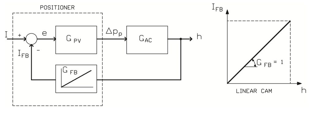
Figure 29. Linear position control.
The behavior of a feedback system can be studied through its transfer function. Figure 29 illustrates the equation (19) for the position closed loop gain.
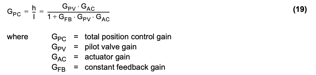
As shown in equation (19), the gain in position control depends on the gains in the individual blocks of the system.
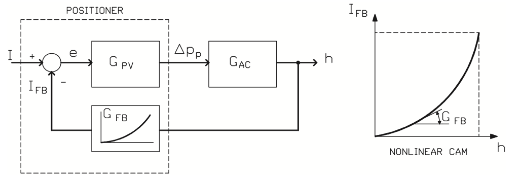
Figure 30. Nonlinear position control.
Figure 30 represents nonlinear position control performed by modifying the positioner feedback cam.
The problem with positioner cam modification is that the correction is made in the mechanical feedback loop of the positioner. Therefore, the correction is made after the point where it was required. Cam modification is thus only suitable for very slow control loops. Moreover, it has the following disadvantages:
- The control valve operates very rapidly in one flow range and very slowly in another flow range, due to the feedback gain (GFB) change with different valve openings (h). In other words, the control loop time constant changes depending on the valve position.
- Control valve position control can become unstable in a certain opening range, due to the stability criterium given in equation (20).
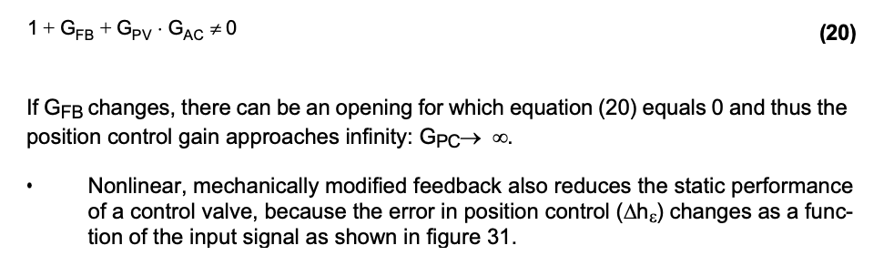
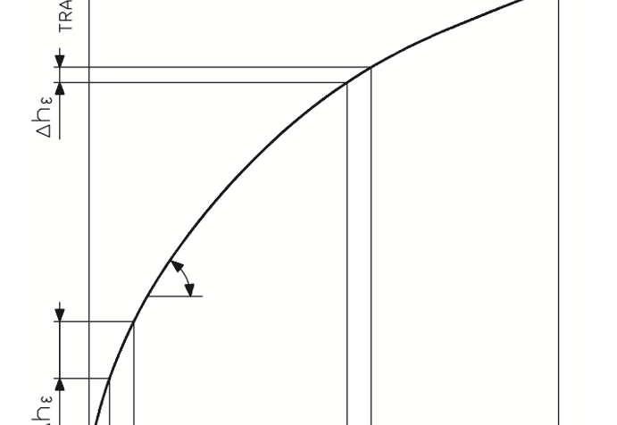
Figure 31. Nonlinear position control error.
If characterization of the control valve is done using controller output modification instead of nonlinear mechanical feedback, the situation changes considerably. It can now be characterized by the block diagram in figure 32.
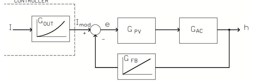
Figure 32. Control valve characterization by controller output signal.
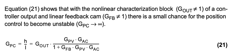
In practice, characterization by modifying the controller output means:
- The installed characteristic modification on the signal level is done very rapidly compared with changes on the pneumatic and mechanical level.
- The error in positioner is constant and does not change according to the opening.
- The chance for position control instability is small.