4 Gas and steam flow
The flow of gas and steam through control valves has been well defined by universal, standardized sizing equations (ISA/IEC). The first half of this chapter is dedicated to giving a description of these equations and the basic fluid mechanics involved in gas or steam flow through control valves.
The second half concentrates on techniques of aerodynamic noise generation, prediction and abatement. This is done for two reasons: firstly, noise is again, after some years of relatively low emphasis, becoming a major environmental issue; and secondly, there is no good, easily understandable literature on the actual generation and abatement mechanics of noise in control valves. The details of aerodynamic noise generation and abatement given here should help explain the reasons for aerodynamic noise generation in control valves, and the different means available for dampening aerodynamic noise.
4.1 General
The main difference of gas or steam flow compared with liquid flow is that in the former, the interrelation of flow and pressure is typically much weaker. A typical pressure source is a manifold with a relatively constant pressure unless the particular process pipe takes a major share of the gas or steam led into it. A typical process installation model for compressible flow, such as a gas or steam flow control valve, is shown in figure 52.
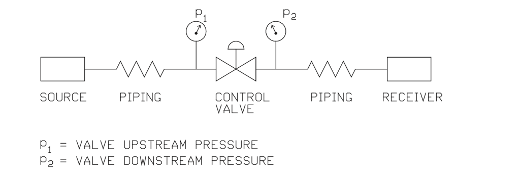
Figure 52. A typical gas or steam control valve installation.
In figure 52, the upstream pressure (p1) is located two pipe diameters upstream of the valve inlet flange, and downstream pressure (p2) is located six pipe diameters downstream of the valve downstream flange (per std. IEC 60534/ISA S75). This chapter concentrates on the throttling process between upstream pressure (p1) and downstream pressure (p2) of figure 52.
The most important difference between liquid and gas flow is compressibility. When the pressure is increased, the volume of the gas decreases, and vice versa. For the flow, constant flow units like mass flow or standard volumetric flow units, are used. The pressure drop ratio x = ∆p/p1 is used instead of pressure drop alone because gas expansion is related to this ratio. The speed of sound is a significant measure of the effects of compressibility compared with the velocity of flow. This introduces a dimensionless parameter which is called the Mach number. The calculation for the Mach number (Ma) is given in equation (48).
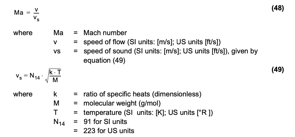
Figure 53 shows the interrelation of flow through a control valve at a constant opening and constant upstream pressure (p1). It shows the flow through a gas or steam valve starting to deviate from a straight line at fairly low pressure drop due to gas compressibility. Accordingly, the valve inlet pressure is higher and the volume smaller than at the outlet where lower pressure causes higher volume. This expansion becomes a significant factor at higher pressure drop ratios (∆p/p1).
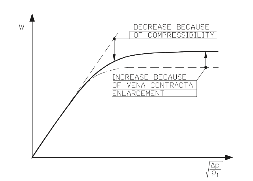
Figure 53. Interrelation of flow and pressure drop ratio in gas or steam valves.
The phenomenon of choking, i.e. a situation in which an increase in pressure drop (∆p) across the valve does not produce an increase in flow, also occurs in gas and steam flows. However, the reason here is different. Whenever the fluid reaches sonic flow velocity at the vena contracta, the smallest actual flow area location, a further increase in pressure drop (∆p) at constant inlet pressure will not increase the flow velocity at the vena contracta, although supersonic velocities may exist downstream of the vena contracta. The flow can still be increased as a result of vena contracta enlargement. When the pressure drop is further increased beyond the sonic velocity at the vena contracta, the vena contracta moves upstream towards the valve orifice and the area of the vena contracta gets larger, therefore increasing the flow. When the vena contracta reaches the physical valve orifice, the flow becomes fully choked, and an increase in the pressure drop will not increase the flow. The terminal pressure drop at which this happens can be calculated using the pressure drop ratio factor of valve (xT) as in equation (50).

4.2 Sizing equations for gas and steam flow
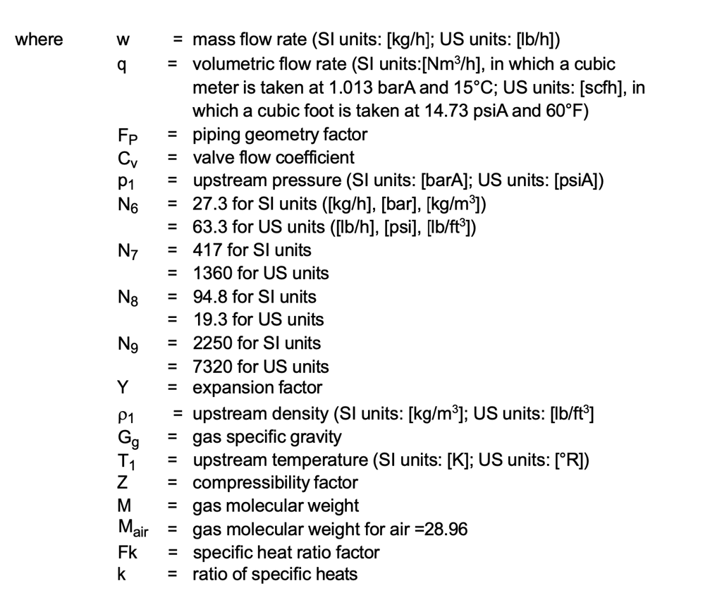
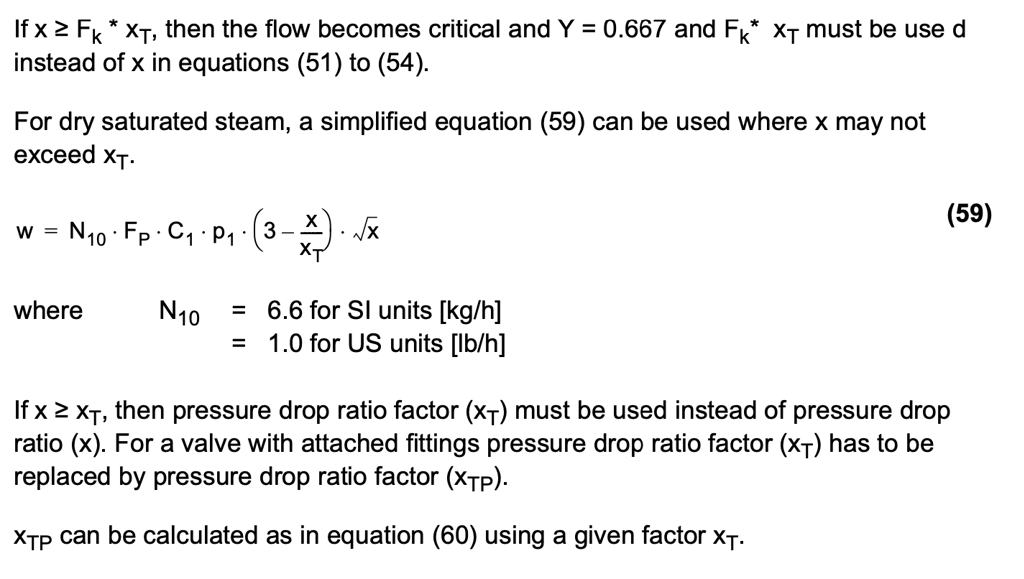
The gas or vapor flow through the valve can be calculated using any of these forms of basic equations (51) to (54).
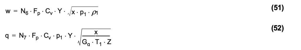
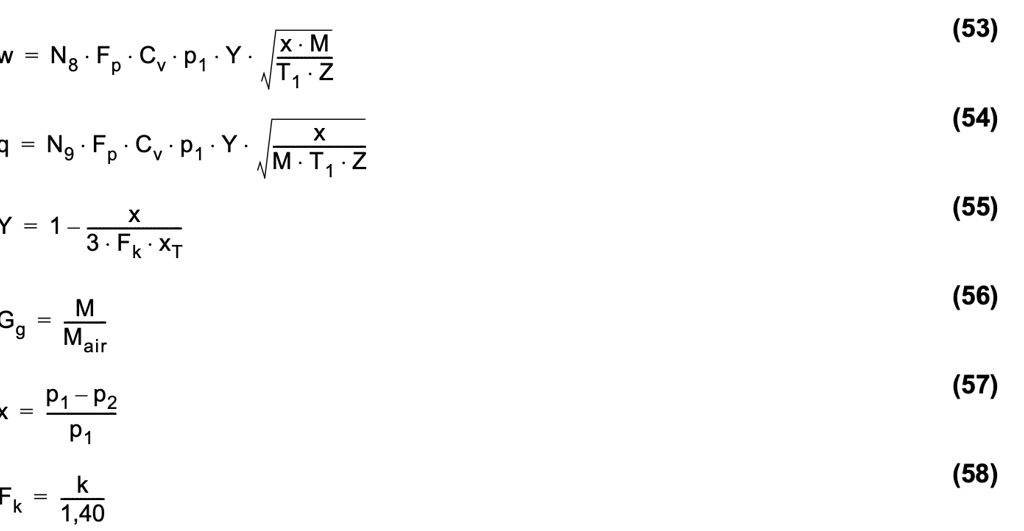
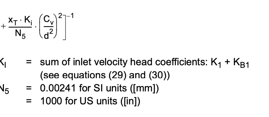
Factor Z is the compressibility factor, and for perfect gas, it has a value of 1.0. In many flows, the fluid behaves as a perfect gas and the compressibility factor (Z) will be 1. The compressibility factor (Z) can be determined from the graph in appendix G as a function of reduced pressure (pr) and reduced temperature (Tr).
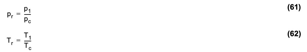
Reduced pressure (pr) is defined as the ratio of the actual inlet absolute pressure to the absolute thermodynamic critical pressure, as in equation (61). The reduced temperature Tr is defined similarly, as in equation (62).
4.3 Aerodynamic noise
4.3.1 Aerodynamic noise generation
The noise created by throttling gas or steam is called aerodynamic noise. Aerodynamic noise at subsonic velocities is generated by three forms of aerodynamic sources: monopole, dipole and quadropole. Aerodynamic monopole noise can be described as a pulsating sphere causing the acoustic pressure waves. This type of noise is typical of pulse jets, sirens and propellers. Monopole sources can also be caused by flow instability. The intensity of noise in this case is proportional to the fourth power of the flow velocity.
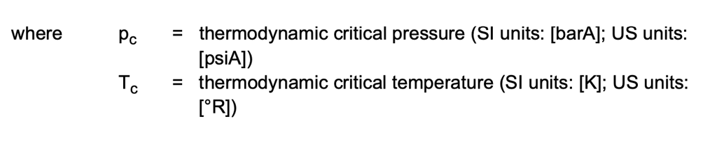
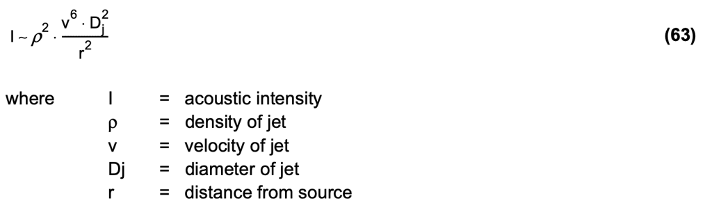
Control valve aerodynamic noise is mainly caused by dipole sources when the flow velocity is subsonic. An aerodynamic dipole consists of two monopoles pulsing 180°out of phase near a solid boundary. In this case, the acoustic intensity is given by the following proportionality equation (63).
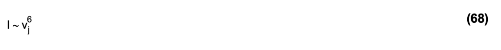
High-speed jet noise is generated by aerodynamic quadropoles which consists of two dipoles pulsing in opposing pairs. According to Lighthill's classic work, the proportionality of noise intensity is, in this case, as in equation (64).
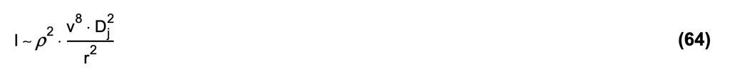
The noise intensity here is proportional to the eight power of the velocity. This applies to a free jet.
In choked flows where the flow velocity reaches sonic velocity, the flow becomes critical, and the main sources of noise are the shock waves and turbulence interactions. Shock waves and turbulence interactions have been found to create a 'screech' from acoustic feedback. Figure 54 describes the change in noise intensity as a function of fluid velocity.
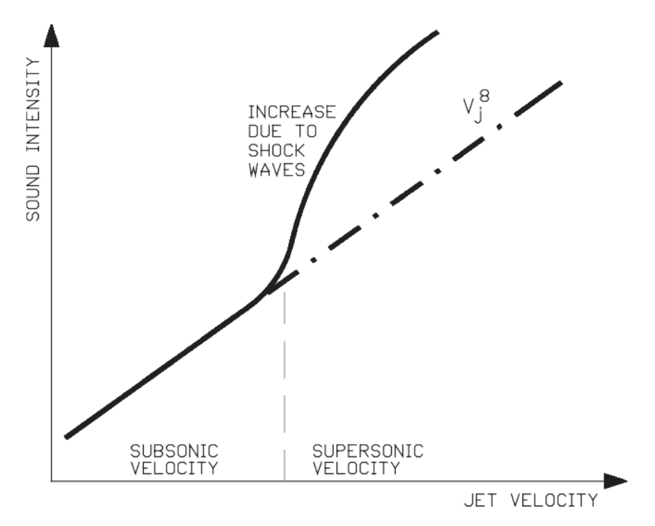
Figure 54. Velocity and jet noise interrelation.
Shock waves which are perpendicular to the free jet stream are called normal shocks or direct shocks. A normal shock is illustrated in figure 55.
The shock wave can also be oblique if the flow passes a wedge or sharp object, or if supersonic flow is forced to change direction by a solid boundary. Figure 56 shows an attached and a detached shock wave.
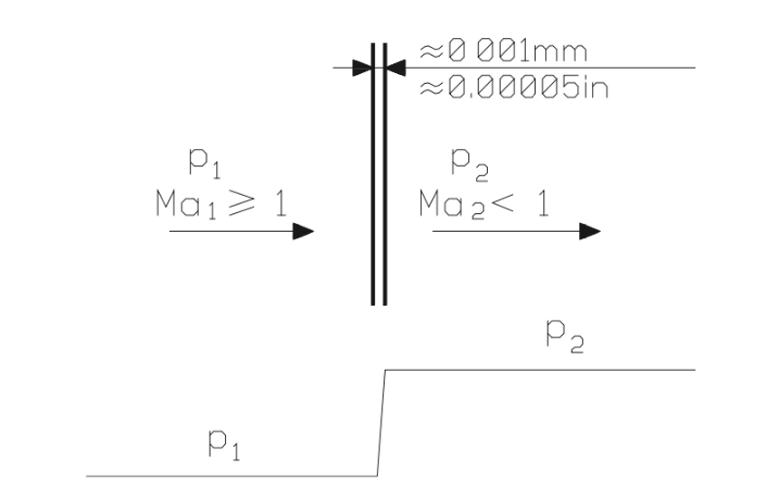
Figure 55. Pressure change in a normal shock wave.
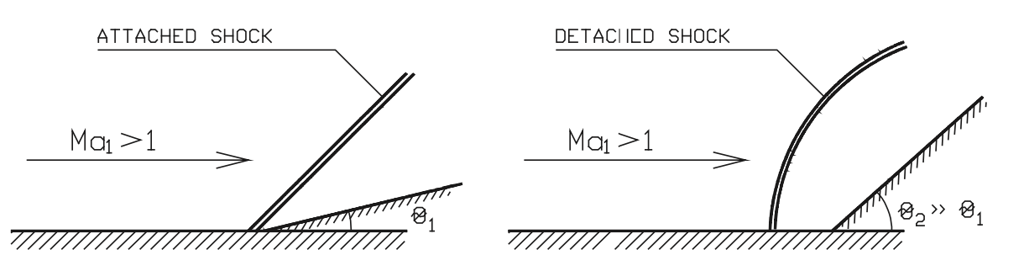
Figure 56. Attached and detached shock waves.
Shock waves can be reflected from solid boundaries and they can penetrate each other. A control valve outlet flow stream can create an oscillating chain of compression shock waves with declining cycles and intensity, as shown in figure 57. This is a very powerful noise source.
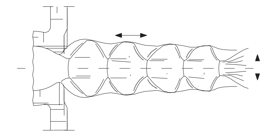
Figure 57. A chain of compression shocks.
With computational fluid dynamics, it is possible to simulate shock waves in different geometries. Super computers are normally used because the calculation requires a great deal of complicated computations.
Figure 58 is a print-out of a calculation with a rotational symmetrical geometry. The lines in figure 58 represent constant pressure regions. The shock waves are where the lines are dense. The results calculated by the state-of-the-art computer programs are used in the design of low noise trims and attenuators.
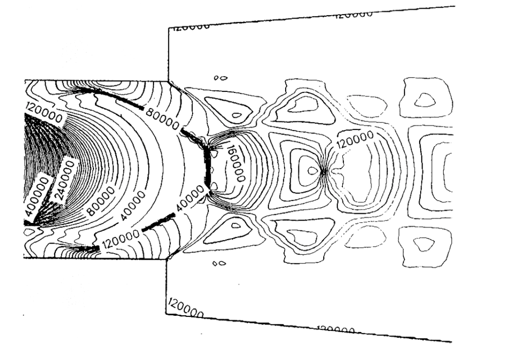
Figure 58. Computational shock wave pattern downstream of rotational symmetrical geometry.
4.3.2 Aerodynamic noise prediction
At low pressure ratios (p1/p2), the cause of aerodynamic noise is turbulence. At high pressure ratios, the flow becomes critical and the turbulent interactions of the shock waves become the major source of noise.
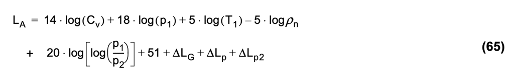
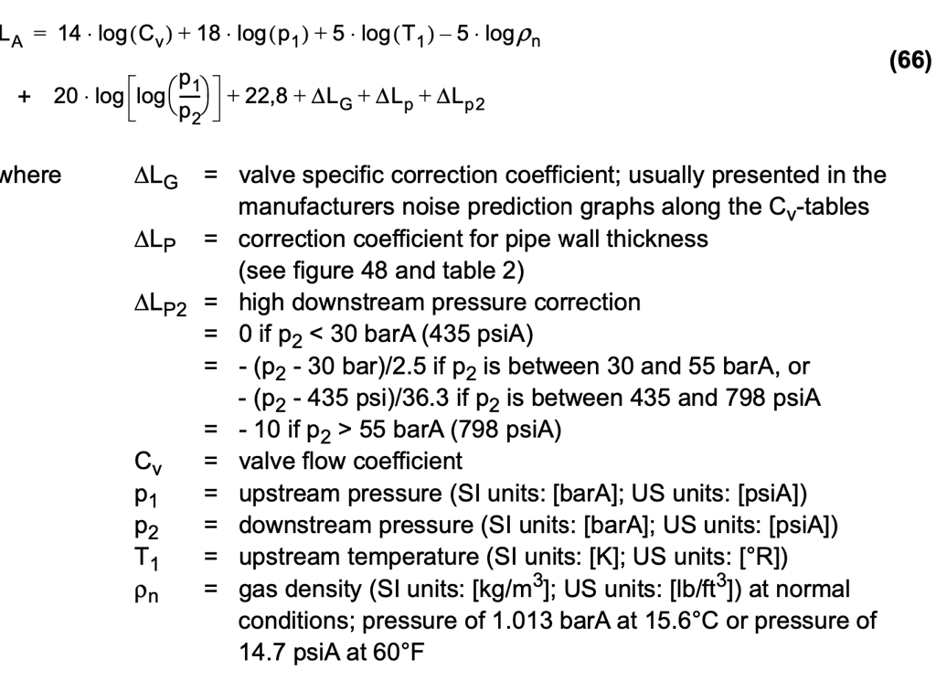
Calculation method to predict aerodynamic noise level
The noise level LA in dB(A) is calculated using the following equation (65) for SI units and equation (66) for US units. Equations are based on VDMA 24422 (1979 version) standard (see appendix K).
Aerodynamic noise prediction according to the IEC 60534-8-3 is very similar to IEC hydrodynamic noise prediction. The noise prediction is based on a similar method where mechanical stream power as well as acoustical efficiency factors are calculated in five different flow regimes. The standard defines regimes as a function of the pressure drop ratio (x). The sound pressure level inside the pipe is estimated and the pipe external noise is attained from inner sound pressure level by reducing the transmission loss of the piping.
Acoustical efficiency factors, peak frequency, and the mechanical stream power calculations depend on the flow regime. Otherwise, the IEC aerodynamic noise prediction has similar steps than in hydrodynamic noise (see steps in chapter 3.5).
Due to the extent of the standard, the manual users are recommended to refer to the IEC 60534-8-3 for details.
4.4 Atmospheric venting
Venting gas or steam to the atmosphere usually generates high noise levels around the vent exit. In such cases, the jet noise inside the pipe is released into the air, generating possible sound pressure levels from 140 up to 170 dBA one meter from the vent exit.
Noise levels of this magnitude are hazardous to the personnel, and in many countries, strict noise abatement laws require action to reduce noise to acceptable levels near the manufacturing facilities.
As a result of high noise level in atmospheric venting, a control valve is normally equiped with a low noise trim. Often a special vent diffuser or vent silencer is required to achieve an acceptable noise level.
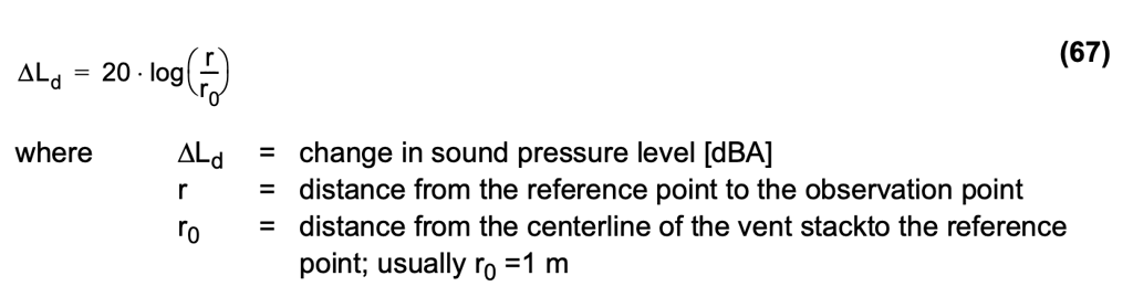
The observation point for vent noise is usually far from the vent exit which can be considered a point noise source, and the sound pressure level decreases as a function of distance, as in equation (67).
When the vent exits are high above ground level, for example, in gas-to-flare applications, the observation direction has a substantial effect on the noise. The directivity effect attenuates the most in the opposite direction of the vent flow, and the least in the direction of the vent flow. Attenuation can be as high as 15 dBA depending on the observation direction.
Further away, in addition to the above reductions, more attenuation can be expected owing to environmental and other conditions such as absorption into the air, attenuation by barriers, vegetation, and topography, or by wind and temperature gradients.
VDMA 24422 (version 1979) only calculates noise in a closed piping system, and there are no standard methods for predicting noise at an open pipe end. That is why noise prediction for an atmospheric outlet uses an empirical method.
4.5 Aerodynamic noise abatement
Abatement of the noise produced in the throttling process can be done in several ways. The basic division of these is between 'source' treatment, i.e. valve and trim modification, so that generation of excessive noise is prevented, and 'path' treatment, i.e. dampening the generated noise.
Source treatment, whenever possible and feasible, is the preferred form of noise abatement. This is because when source treatment is used, the high mechanical vibration levels always associated with noise can be prevented, thus ensuring reliable operation of the process.
A combination of source and path treatment often provides the most economical sound dampening system. Figure 59 shows the basic options for aerodynamic noise abatement.
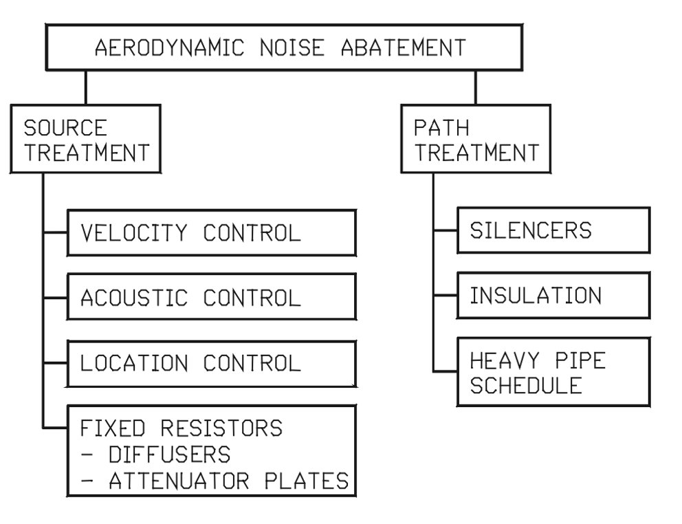
Figure 59. Options in aerodynamic noise abatement.
4.5.1 Source treatment
Source treatment of noise, i.e. preventing the generation of excessive noise levels, can be performed by at least four different methods: velocity control, acoustic control, location control, and using diffusers.
Velocity control
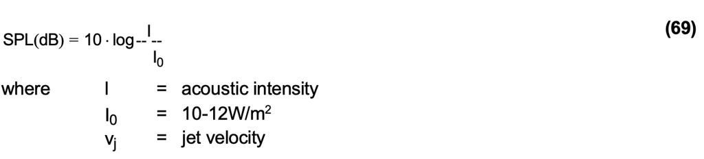
Controlling the maximum fluid velocity inside a control valve trim is a very effective way of controlling noise at sub-sonic flow velocities in the trim, as the acoustic intensity of a jet has been shown to be proportional to the sixth power of the flow velocity in a system with solid boundaries like a valve trim or a pipe. The relation between sound pressure level (SPL) and acoustic intensity is given in equation (69).
The control valve trim velocity can most effectively be controlled using a multistage pressure drop, and by increasing the valve trim outlet area such that the flow velocity and pressure at the valve outlet are the minimum and the gas volume the maximum. Figure 60 illustrates the basic principle of a staged pressure drop.
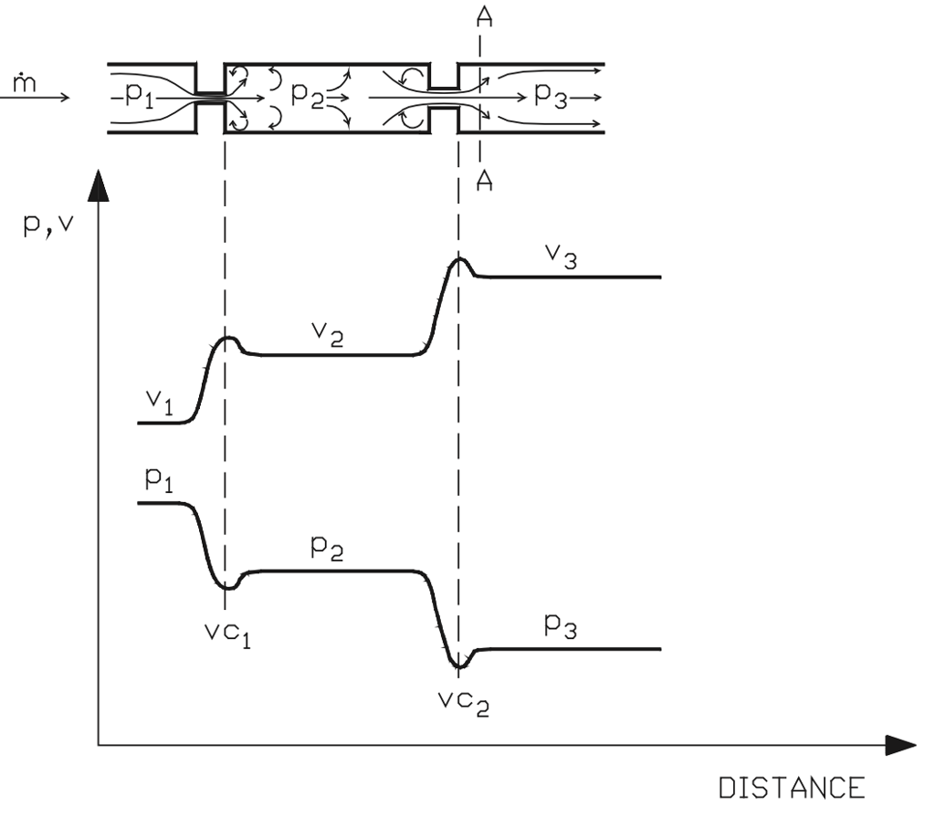
Figure 60. Effect on flow velocity of a multi-stage pressure drop.
When the pressure drop across a control valve is taken in multiple stages, as in figure 59, the total pressure drop (p1-p31) is divided into several smaller successive pressure drops (p1-p2, p2-p3). The successive stages are spaced in such a way that the gas pressure is allowed to recover to an intermediate pressure (p2) and velocity (v2) before the next throttling stage. This intermediate recovery of pressure and the resulting velocity reduction prevent the fluid from reaching the velocity it would have in a single-stage pressure drop system. In other words, the smaller the pressure drop, the smaller the recovery and fluid velocity increase downstream of the orifice. An infinite number of stages would, therefore, produce a valve with no pressure recovery, in which the velocity at the vena contracta would equal the downstream velocity. However, economics and mechanics limit the number of stages actually used in valves. Note that an expanding flow area is used for each successive stage in gas processes to counter the expansion of the gas as the pressure drops.
Acoustic control
Acoustic control affects the noise level by means of acoustics. Two methods used in control valves are described here: flow division into multiple streams, and the modification of acoustic field.
In theory, as given by equations (63) and (64), flow division into multiple streams is effective because the intensity of noise generated by a single orifice decreases rapidly when hole diameter is decreased. Thus a number of small holes attenuates noise more effectively than one big hole. A rule of thumb is that each doubling of the number of holes reduces noise by 3 dB, as illustrated in figure 61.
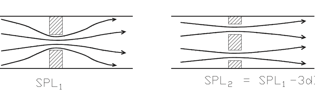
Figure 61. Effect of increasing number of holes on noise level.
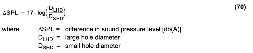
In practice, increasing the number of flow passages by making them smaller also affects the noise frequency distribution. Equation (70) is an experimental equation showing the noise reducing effect of smaller orifices.
The smaller the passage, the higher the noise frequency. High-frequency noise is easily attenuated by the pipe wall, and does not contribute to the 'A'-weighted sound pressure level scale (figure 62). High frequencies also extend beyond the capabilities of the human ear.
Modification of the acoustic field directs the flow path in such a way that the peak noise field is broken up in a more diffused space. Figure 63 gives the values for a dynamically balanced butterfly valve as an example of acoustic field modification.
Figure 63 shows a typical acoustic field for a conventional butterfly valve (top of the picture), and for a noise and cavitation attenuating equipped butterfly valve which diffuses the checkered acoustic field.
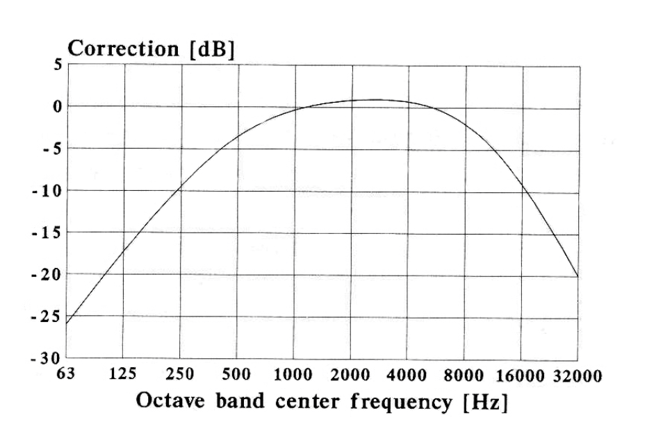
Figure 62. A-weighted sound pressure curve for human ear.
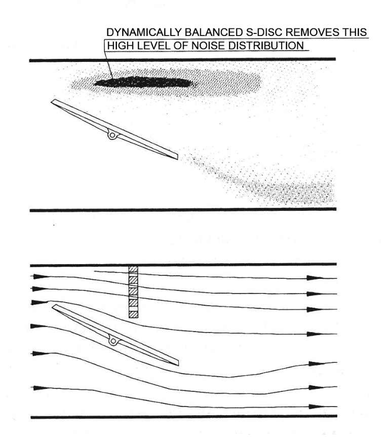
Figure 63. Modification of acoustic field in a dynamically balanced butterfly valve.
Location control
Location control involves designing a valve trim in such a way that the location and the shape of the jet streams in the valve trim, and especially leaving the valve trim, are such that the minimum noise is produced.
There are twomajor sources of noise that can, to an extent, be controlled y intelligent valve trim design. These include the formation of turbulence in the mixing region between where the jet exits from an orifice and the gas flow at the outlet region, and the attachment and interaction of shock waves (generated during throttling if the flow reaches sonic velocity in the valve) One way to do this is to smooth the velocity profile of the jet by introducing a lower velocity gas stream alongside the jet, as shown in figure 64.
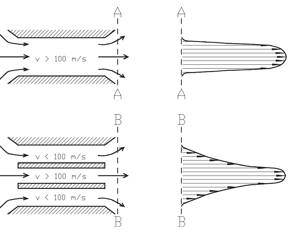
Figure 64. Jet velocity profile modification.
Other methods include using orifice shapes and spacing orifices to ensure that the shock wave interactions generate the minimum amount of total noise.
Diffusers
Dividing the pressure drop between a control valve and a downstream diffuser provides an effective way of further increasing the noise attenuation in cases where there is a constant, high pressure drop across the control valve and the flow rate is relatively constant. Diffusers are fixed area flow resistances and are custom-made for a particular flow condition.
A high pressure drop over the valve generally causes noise and vibration problems in the gas and steam flow. An inline diffuser is a constant area flow resistance used at the valve outlet to increase valve downstream pressure.
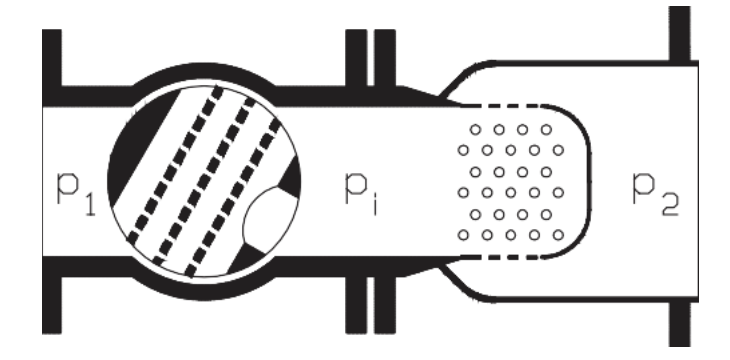
Figure 65. Valve with single stage diffuser.
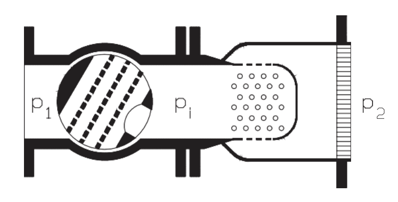
Figure 66. Valve with double stage diffuser.
Software tools are available for sizing diffusers.
It is recommended that a single-stage diffuser be used when the pressure drop ratio (p1-p2)/p1 under maximum flow conditions is higher than 0.65, and a double-stage diffuser when the ratio exceeds 0.75. These recommendations are for valves equipped with noise attenuating trims. In the case of a standard valve with a diffuser and a pressure drop ratio (p1-p2)/p1 smaller than 0.65, a different arrangement may be needed.
Depending on the type of diffuser, single or double-stage, it is recommended that the pressure differential (p1-pi) across the valve be set according to the graphs in figure 67.
The pressure differential (p1-pi) is set for flows in which the highest capacity (Cv) is needed for the valve. The capacity (Cv) of the diffuser is calculated under maximum flow conditions using equations (51) to (54). Intermediate pressure (pi) and corresponding density (ri) are used as upstream pressure and density. The pressure drop ratio factor (xT) is 0.5 for a single-stage and 0.7 for a double-stage diffuser. The capacity (Cv) of the diffuser remains constant, and this is used to calculate (p1-pi) and the intermediate pressure (pi) for other flow conditions.
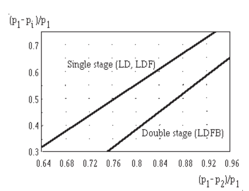
Figure 67. Pressure differential selection for line diffuser.
In noise calculations, the noise from the valve and diffuser are first calculated separately using the standard VDMA 24422 noise prediction method. The intermediate pressure (pi) is the valve downstream and diffuser upstream pressure. The noise level of the total package is achieved by summing both noise levels logarithmically. A 6 dBA insertion loss is subtracted from the valve noise level, and the total noise level is then given by equation (71).
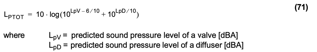
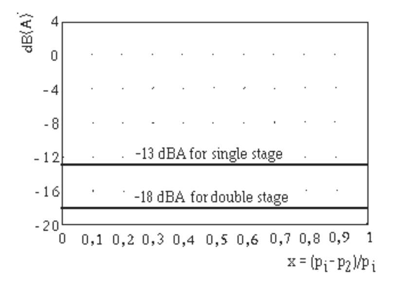
Figure 68. Aerodynamic noise coefficient ∆LG for diffusers as a function of pressure drop ratio (x), as x = (pi-p2)/pi.
The outer shell diameter of the diffuser is normally sized to match the downstream piping. However, the flow velocity in the annular area between the inlet tube and the outer shell of the diffuser should not exceed 0.5 * vs if regenerated noise caused by high flow velocity is to be prevented.
The minimum outer shell diameter to meet this requirement is given by equation (72).
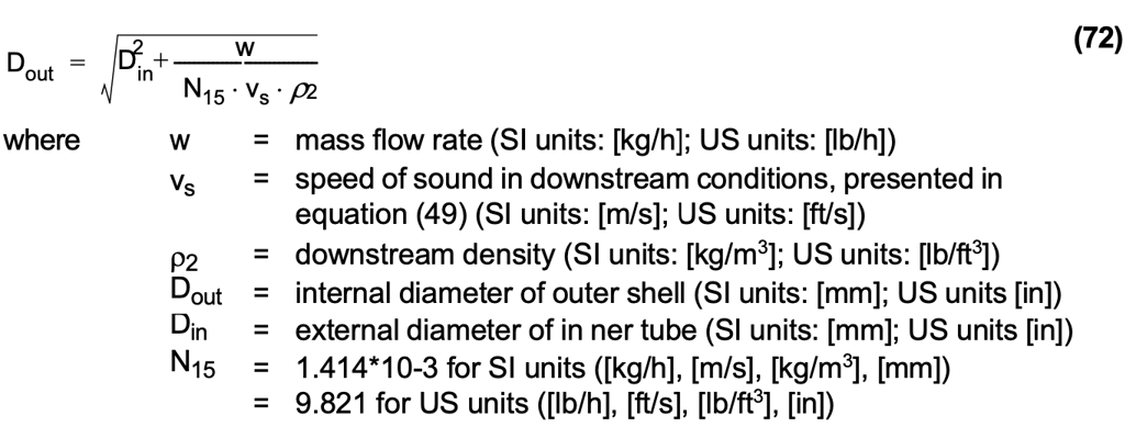
A smaller outlet shell than calculated from equation (72) can be used if, for example, the outlet shell should be the same size as the downstream pipe. In these cases, it must be taken into account that flow velocity in the annular area will be greater than 0.5 * vs, resulting in limited diffuser noise reduction capability for the diffuser.
When the outlet shell specified by equation (72) is bigger than the downstream piping, the reduction of the downstream pipe can begin straight after the end of the diffuser inlet tube.
Attenuator plates
Dividing the pressure drop between the valve and a downstream device provides an effective methods noise attenuation in cases where the pressure drop is close to constant across the valve. An attenuator plate is a fixed restriction installed downstream of the valve, as shown in figure 70.
High pressure drop across a valve generally causes noise and vibration problems in the gas and steam flow. An attenuator plate is a constant-area flow resistance used at the valve outlet to increase valve downstream pressure. Noise attenuation is achieved by specific hole geometry. This hole geometry is a result of computational and experimental studies. Figure 69 is a printout of a calculation of the flow through one hole in an attenuator plate. The lines in figure 68 represent constant density regions.
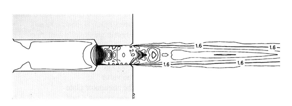
Figure 69. Constant density regions of flow through a hole in an attenuator plate.
The attenuator plate capacity is fixed for each nominal size. If a higher capacity is needed, the nominal size of the attenuator plate has to be increased. Normally the nominal size must be selected between the valve and downstream pipe diameter. Pressure and flow conditions with the selected plate are calculated using standard ISA/ IEC sizing equations.
The attenuator plate is mounted between flanges downstream of the valve. Mounting can be between the valve and pipe flanges or between piping flanges. For some valves, an attenuator plate is also available as an integrated unit inside the valve body.
Mounting the attenuator plate between the valve and pipe flanges is not allowed if the valve is a butterfly valve or flangless segment valve, or if the attenuator plate is already integrated into the valve body. In these cases, at least one pipe diameter of pipe is required between the valve and the attenuator plate.
The attenuator plate is usually effective for noise reduction when the pressure drop ratio (p1-p2)/p1 is less than from 0.8 to 0.9, depending on the valve type and opening. A diffuser is recommended for higher pressure drop ratios.
The pressure differential across the attenuator plate is calculated for each flow according to basic gas sizing equations. The intermediate pressure (pi) is iterated from equations (51) to (54), replacing upstream pressure (p1) with intermediate pressure (pi). Sizing is most easily done with sizing and selection software. The critical pressure drop ratio for an attenuator plate is 0.39. Cv is obtained by selecting the nominal size of the attenuator.
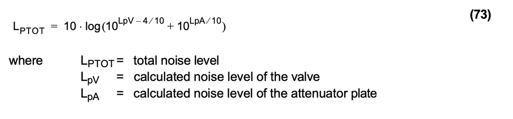
Noise calculations for the valve and attenuator plate are first performed separately using intermediate pressure (pi) as both the valve downstream and the attenuator plate upstream pressure. The noise level of the total package is found by summing both noise levels logarithmically. A 4 dBA insertion loss is subtracted from the valve noise level. The total noise level is then as given in equation (73).
Source treatment examples
Source treatment is demonstrated using rotary type noise control trim valves, such as in figure 70.
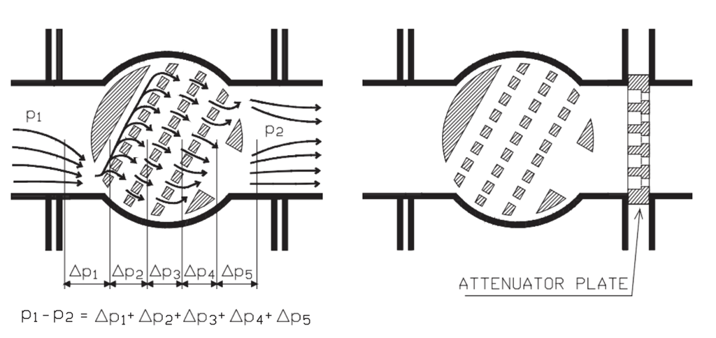
Figure 70. A noise control trim provides a combination of effects for reducing noise level in gas controlling applications; on the right, an attenuator plate is installed between valve and pipe flanges.
These noise control trims use a combination of the effects listed in the following paragraphs:
-
The trim velocity is minimized using a multistage pressure drop. Trim outlet velocity is minimized by opening up the downstream cheek of the trunnion mounted ball valve or by using segment valves with no restriction at the trim outlet.
-
Division of the flow into multiple streams in attenuator holes attenuates the noise following the principles of acoustic control.
-
The trim outlet is designed to provide a uniform acoustic field in the valve outlet port, thus minimizing disturbances with creating high-noise areas in the acoustic field.
The rotary motion of these valves has the additional benefits of allowing very large flow ranges and the passing of impurities through the valve.
4.5.2 Path treatment
The path treatment of noise, i.e. suppressing the transmission of excessive noise levels, can be performed by using least three different methods: silencers, insulation, and heavier pipe schedule.
Silencers
Silencers are mufflers used in-line or at an outlet to the atmosphere to dampen the noise produced. Reactive silencers create frequency interactions to dampen noise, whereas dissipative silencers use sound-absorbing materials like glassfibre to dampen the noise.
The main use for silencers is on atmospheric outlets for gas or steam. In such cases, the jet noise inside the pipe is released to the open air, and very high noise levels can easily develop. Typically, a combination of reactive and dissipative methods are used in atmospheric vent silencers.
Insulation
Pipe insulation may be used to dampen noise in gas and steam lines, particularly in steam lines where there is already thermal lagging. Thermal insulation can dampen noise 1–2 dB(A) per 10 mm of insulation thickness (3 to 5 dB(A) per inch). The practical maximum is about 12 dB(A) due to leaks and acoustic bridges. Special acoustic insulation reduces noise up to 4 dB(A) per 10 mm of insulation thickness (10 dB(A) per inch). The maximum attenuation for acoustic insulation is 20–25 dB(A).
Two things should be noted in using insulation for dampening noise: Firstly, a noise level greater than 100 dB(A) should primarily be handled by source treatment methods to avoid hiding potential vibration damage by insulation. Secondly, the true cost of installing acoustic insulation should be calculated before using it for long pipelines. This is because noise is attenuated very slowly in piping filled with gas or vapor, and because long pipe runs may have to be insulated in order to achieve acceptable noise reduction.
4.6 Recommended flow velocities and limits for noise levels
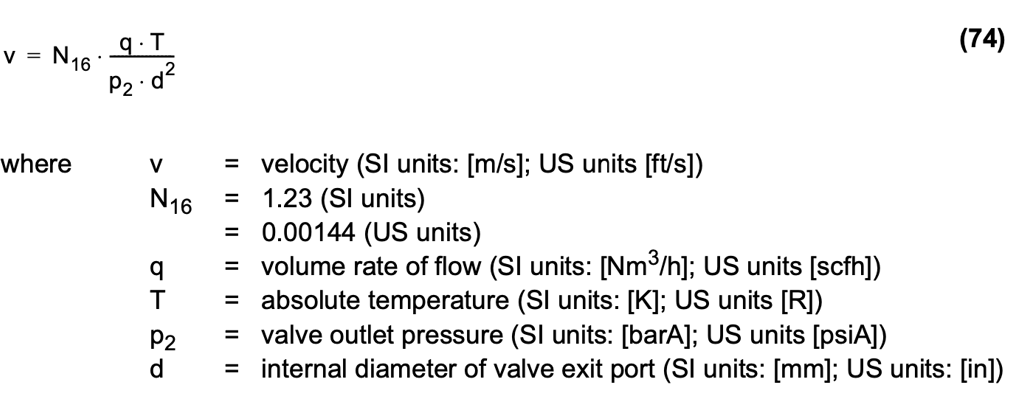
The flow velocity for gases or steam downstream of the valve can be calculated as in equation (74).
The recommended flow velocity at the valve exit port is given in terms of sonic velocity, as in inequality equations (75) and (76).
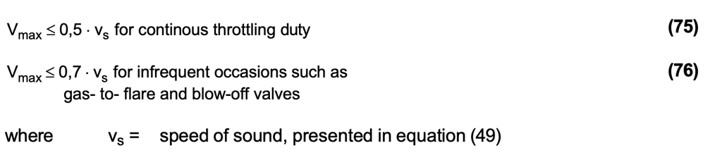
Naturally, the above velocity limits are for relatively pure gases and steam. In the case of impurities in the flow or wet steam, the flow velocities need to be lowered to prevent erosion damage.
To prevent mechanical damage of a valve and to ensure operation of control valve instrumentation, it is recommended that sound pressure levels (SPL's) exceeding 110 dBA (calculated with uninsulated Schedule 40 piping) are never used.