6 Mathematical simulation of control valve behavior

6.1 General
The use of computational science has resulted in a control valve simulation program that can be used to describe the dynamic behavior of control valves.
6.2 Use of simulation
Use of simulation can be divided into three areas:
-
In development of new products.
-
In support for customer's process applications.
-
In training of personnel about fluid flow control and control valves.
In the development of new products, simulation can be used to test new ideas, and to develop and optimize constructions before a prototype is manufactured. Simulation thus reduces the number of prototypes required. It can also be used to study the effects of different disturbances on control valves.
Before the delivery to a customer, the operation of a control valve packages can be simulated in conditions that equal the real process conditions. Simulation makes it possible to study the operation of the whole control loop including the customer's process. The simulation program can also be used to study various questions relating to the safety of process plants.
When training the personnel in the area of control valves, simulation can be used to illustrate the operation of different control valve units in process pipelines. In addition, simulation makes it possible to examine different control valve characteristics in the whole control loop.
Simulation of customer's control applications is a state-of-the-art service designed to study the control valve dynamic behavior before delivery. A detailed dynamic analysis performed in simulated process conditions enhances the optimal control valve selection for customers' demanding control valve applications.
6.3 Mathematical model of a control valve
The starting point for the control valve simulation program is a comprehensive mathematical model describing the operation of the control valve, right from the control signal from the controller to the fluid flow through the valve.
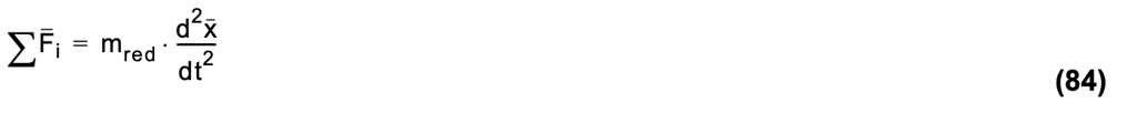
The dynamics equation of a quarter-turn control valve can be found using the basic equations (84) and (85).
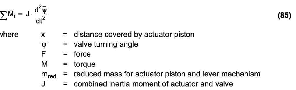
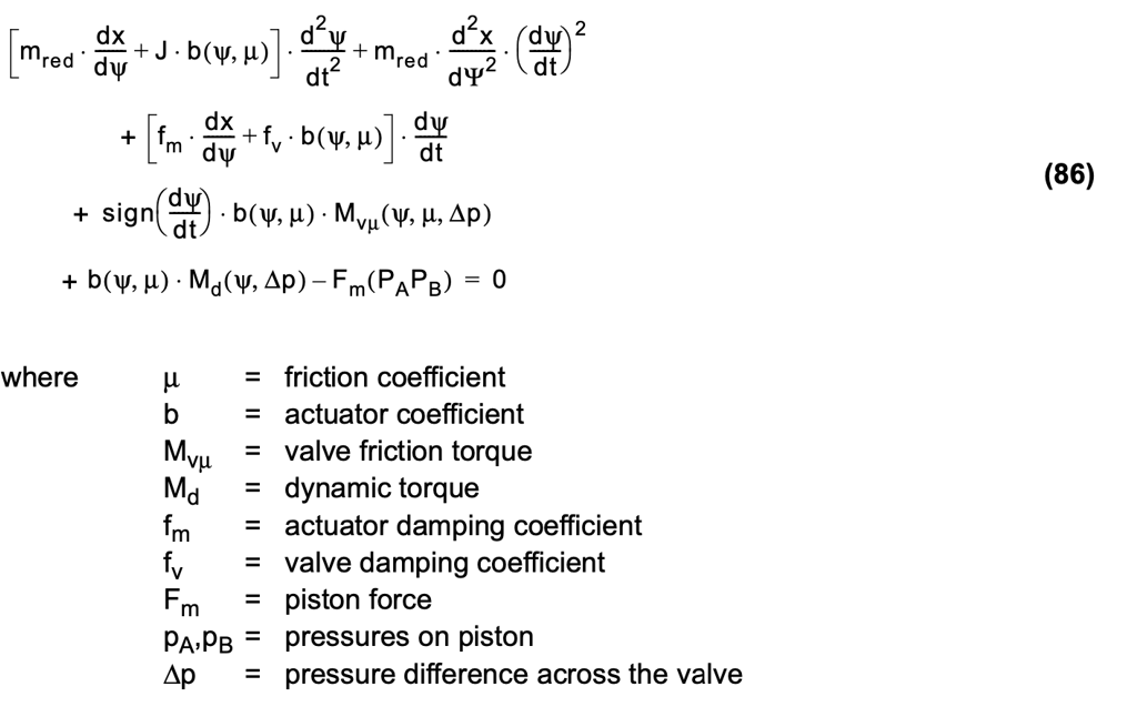
Equations (84) and (85) can be used to produce the equations for the dynamics of an installed quarter-turn control valve as in equation (86).
The actuator coefficient (b) used in equation (86) is a function of the actuator turning angle (ψ) and friction coefficient (μ). Figure 74 shows the actuator coefficient for one manufacturer's actuator as a function of actuator relative travel (h) when the friction coefficient (μ) is assumed to be constant.
The non-linearity of the actuator coefficient (b) depends on the lever mechanism of the actuator. In practice, actuator friction coefficients vary greatly as a function of velocity. This means that in reality, the actuator coefficient is less linear than indicated in figure 74.
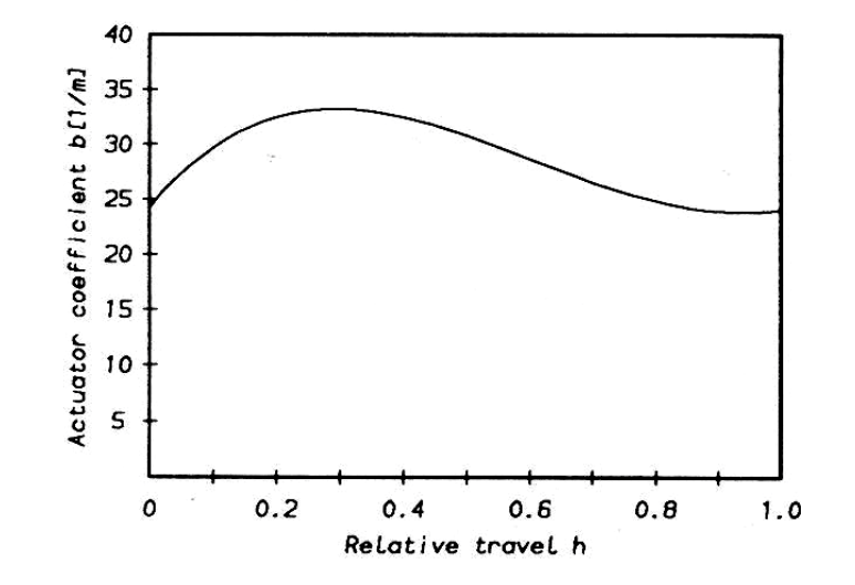
Figure 74. Actuator coefficient of the actuator examined.
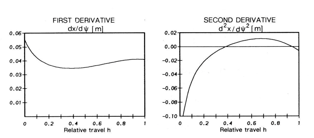
Figure 75. Derivatives in equation (86) as a function of relative travel
Figure 75 shows the non-linearity of the derivatives in equation (86) for the actuator examined, as a function of actuator relative travel (h). The first derivative in figure 74 describes the non-linearity between the actuator piston position (x) and the valve turning angle (ψ). The non-linearity of the derivatives depends on the lever mechanism of the actuator.
As the control valve dynamic equation (86) includes pressures pA and pB, affecting both sides of the actuator piston, they must be solved from the mathematical models describing positioner dynamics and actuator thermodynamics.
In equation (86), the valve load has been divided into the load caused by friction (Mvμ) and the load caused by dynamic torque (Md), since the dynamic torque usually tends to close the valve. The valve load consists of the seat friction, gland packing friction, bearing frictions, and dynamic torque of the valve. A mathematical model is needed to solve these torques as a function of valve travel (h) and the pressure difference (∆p) across the valve throttling element. Because the pressure difference (∆p) over the throttling element changes considerably in a control situation, especially with large travel changes, the mathematical model of the control valve must include a dynamic model of pipe flow.
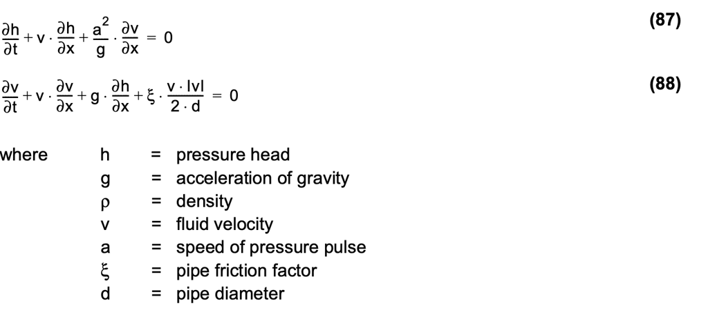
Unsteady pipe flow control is calculated using the continuity equation (87) and the equation of motion, equation (88).
6.4 Control valve simulation program
The solution of mathematical models describing control valve action in space-time is not, however, mathematically possible as such, because the equations are complicated and nonlinear. For this reason, a numerical solution produced by a computer program has to be adopted. One advantage of the computer program is that the non-linearities in the control valve do not have to be linearized. Furthermore, the computer program is flexible because different changes and disturbance factors, depending on time and state, are easy to insert.
6.5 Friction model
A large decrease in the friction coefficient right after the valve starts to move is an important factor in the dynamics of a control valve equipped with a pneumatic cylinder actuator. This means that the correct modeling of friction behavior is decisive for proper functioning of the simulation program.
Lubrication mechanisms can be divided into contact lubrication and fluid lubrication. In contact lubrication, the sliding bearing surfaces touch each other, although the lubricant limits the contact area by penetrating between the contact points. In fluid lubrication, the pressure generated in the bearings prevents any contact between surfaces, and the friction force is created only by the shear stress of the lubricant.
The starting point for the contact friction model used is the exponential friction model, in which the friction force depends exponentially on relative slide velocity (vr). Applying the model gives the equations (89) and (90) for the contact friction coefficients.
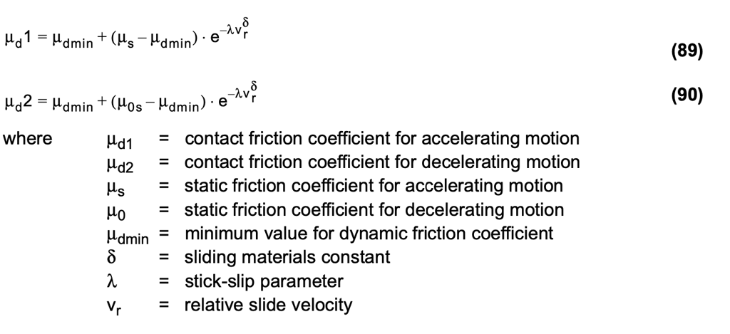
The control valve friction model can be determined by approximating the contact friction, using the exponential friction coefficient, and by assuming that the fluid friction is directly proportional to velocity.
6.6 Testing and implementing the simulation program
Testing position control
The created simulation program was first tested with a single-stage pneumatic positioner, a double-acting cylinder actuator, and a valve with a load factor (Lp). In this case, the actuator load factor (Lp) is the valve load divided by the actuator nominal output torque. Figures 76 and 77 show one form of step response calculated with the simulation program, and the corresponding valve relative travel (h) measured when the relative input signal (I) changes from value 0.4 to value 0.45. As becomes apparent from the step responses presented in figure 76, the form of the response calculated theoretically using the simulation program is fairly consistent with the corresponding response measured in a laboratory by means of an oscilloscope.
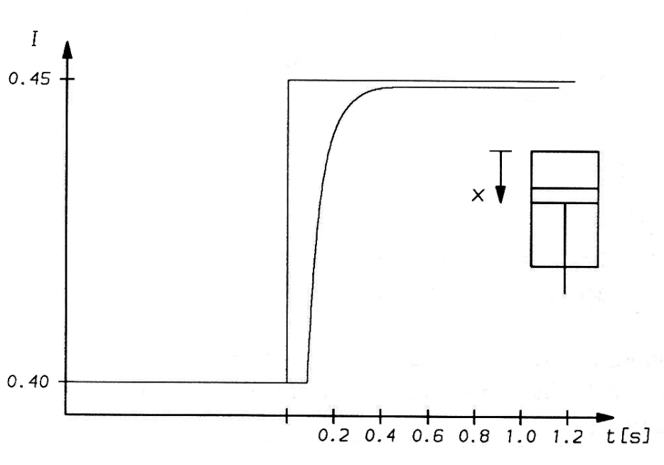
Figure 76. Step response calculated theoretically with the simulation program when the value of the relative signal changes from 40% to 45%.
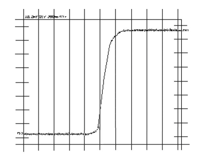
Figure 77. The corresponding step response measured in the laboratory using an oscilloscope.
Studies of an installed control valve
Figure 78 shows a preliminary study of a water-hammer with three different inherent flow characteristic curves. The calculations are based on a single-stage pneumatic positioner, a double-acting cylinder actuator and linear, equal percentage, and constant gain inherent flow characteristics.
The characteristic pressure difference ratio (DPf) describing the pipeline is determined using equation (91).
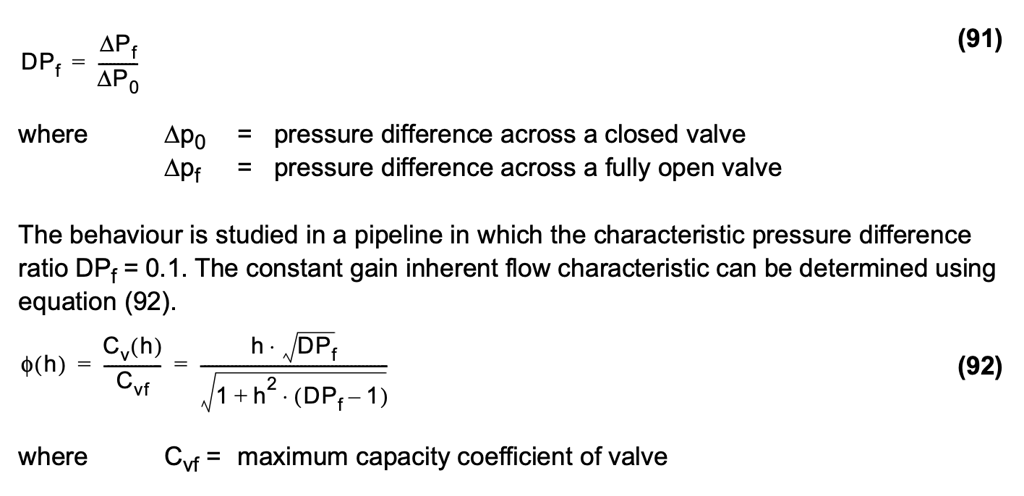
The starting point for the case is a constant gain inherent flow characteristic valve which performs the signal change from 100% to 10%. For the equal percentage opening valve with a corresponding steady-state pressure difference and flow rate change, the signal change is from 100% to 12.0%. For a linear valve, the corresponding signal change is from 100% to 3.2%.
Figure 78 shows that the water-hammer caused by a valve with a linear inherent flow characteristic is very strong and sharp. With equal percentage and constant gain inherent flow characteristics, water-hammers are considerably smaller. Note that in the contant gain inherent flow characteristics, the change in flow rate is almost linear as a function of time.
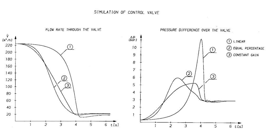
Figure 78. Water-hammer caused by a valve with different inherent flow characteristics.